TECHNOLOGY EXPLAINER
Magnetocaloric Effect and Magnetic Refrigeration
— heating a magnet with a field is easy; what is hard is an effect that does not fade with repetition, and the temperature span a refrigerator needs
A magnetic material warms when a field is applied and cools when it is removed. Magnetic refrigeration, which uses this magnetocaloric effect, has been studied for almost fifty years since the first experiment in 1976 as a way to cool without a compressor or a fluorinated refrigerant. It has still not become a product, because the size of the effect in the material is not the only thing that decides the outcome. This article sets out, within the range of primary sources, the principle of the effect (ΔS and ΔTad), the differences between gadolinium, La-Fe-Si, Mn-Fe-P-Si and Heusler alloys, the problem of first-order transitions and hysteresis, the active magnetic regenerator (AMR) cycle, how far prototype machines have got, and the comparison with thermoelectric, elastocaloric and electrocaloric cooling. Comparisons are read with the field, the temperature span and the sample form held the same.
- What magnetic refrigeration is (the short version)
- The principle — ΔS, ΔT ad and the theoretical upper limit
- Candidate materials — Gd, La-Fe-Si, Mn-Fe-P-Si, Heusler alloys
- First-order transitions and hysteresis
- The AMR cycle, and the difficulty of giving the material a shape
- Where prototypes stand — the shift of field source, and the wall of temperature span
- Comparison with solid-state cooling — on equal terms
- Resources and supply
- Limits, and what could not be confirmed
- How to read evaluations and standards
- Glossary
- References (primary sources)
- Claim-to-source audit
Sourced = stated in published material (link given)
Our calculation = a figure this article derived, with the assumptions spelled out
Not yet confirmed = a company plan, a theoretical estimate or a suspended measure whose record has not been confirmed
Materials-design interpretations are marked separately as Commentary. Inference is shown in bold. Regulations and measures are described by distinguishing announcement, entry into force and suspension.
Magnetocaloric numbers change greatly with the size of the field change (1 T, 2 T or 5 T), the method of measurement (direct or indirect), the sample form (bulk or powder) and the temperature. This article gives these alongside each value. Values for prototype machines are the maxima reported for prototypes, not the performance of production units. Cooling power, temperature span and efficiency need not come from the same operating point, so placing the values of different machines side by side does not show which is better. Company plans are marked “not yet confirmed”, and prices and price forecasts are not covered.
1. What magnetic refrigeration is (the short version)
- Principle: when a field is applied to a magnetic material, the magnetic moments line up and the entropy falls, so the temperature rises if the process is adiabatic (and it cools when the field is removed). This is the magnetocaloric effect, expressed as the temperature change ΔTad and the isothermal entropy change ΔSSourced [Source 2]
- The difficulty: for materials near room temperature, ΔTad in a 1 T field change is only about 2–4 K, which falls far short of the temperature difference a refrigerator needs (about 49 K). So the “active magnetic regenerator (AMR)” cycle is used to store the effect in a regenerator and build the temperature difference up. It is a question of the design of the whole system: material, magnet, heat exchange and the way the fluid is movedSourced [Sources 2, 3, 4]
- Where things stand: more than 40 prototypes are reported, and in 2015 a jointly developed wine-cooler prototype was announced, but no commercial product could be confirmed in this article. Large hysteresis, the difficulty of shaping the material into a regenerator, and the cost of the field source are named as the remaining wallsSourced [Sources 2, 4, 9]
A magnetocaloric material is judged not by whether ΔS is large but by whether, under the field change that is actually available, it gives a ΔTad that does not fall off with repetition. And for a machine, the question is not how large an effect there is but how large a temperature difference can be made, and how efficientlySourced [Sources 1, 2, 4].
2. The principle — ΔS, ΔTad and the theoretical upper limit
Gutfleisch et al. define the magnetocaloric effect as the reversible change of a sample’s temperature and entropy with a change of external field. If the field is applied adiabatically the total entropy stays constant; the magnetic entropy falls, the lattice entropy rises by the same amount, and the temperature goes up (ΔTad). If the field is applied isothermally, heat Q = TΔSm moves between sample and surroundingsSourced [Source 2]. Sandeman writes this in continuum thermodynamics: ΔS(T, Hmax) = ∫(∂M/∂T)H dH and ΔTad(T, Hmax) = ∫(T/Cp)(∂M/∂T)H dH [Source 1]. The effect is large near a transition where the temperature dependence of the magnetization (∂M/∂T) is large.
Magnetization is an easy quantity to measure. For that reason many papers obtain ΔSm from isothermal magnetization measurements through the Maxwell relation (the indirect method). Gutfleisch et al. state that “a large ΔSm is not a sufficient condition for a good magnetic refrigerant”, and point out that direct measurements of ΔTad are scarce [Source 2]. Sandeman says that, allowing for the losses of a real regenerator, a ΔTad of at least 1 K in the 1 T available from permanent magnets is the minimum guide for a refrigerant [Source 1].
From an idealized model of a first-order transition, Sandeman derives the maximum ΔTad as (Msat·T·μ0Hmax / Cp)1/2 [Source 1]. For Fe-Rh, using Msat = about 120 A·m²/kg, a formula weight of 159 and Cp = 6R (R is the gas constant), Cp = 6 × 8.3145 ÷ 0.159 = about 314 J/(kg·K). Our calculation With T = 300 K (a room-temperature example) and μ0Hmax = 2 T, the limit is about 15 K, which agrees with the 15 K given in the paper. For 1 T it is about 11 K (√(120 × 300 × 1 ÷ 314)).
The direct measurement for Fe49Rh51 is 12.9 K at 1.95 T, about 86% of the 2 T limit (12.9 ÷ 15.1). The 3.6 K converted to 1 T, on the other hand, is about 34% of the 1 T limit [Source 2]. Sandeman says the ΔTad of most materials is about 4–7 K at 2 T, far from the theoretical optimum [Source 1].
Assumptions and limits: an idealized first-order model with temperature and Cp taken as constant. It was checked only against Fe-Rh data and is not an upper limit for other materials. The conversion to 1 T is a value that is not necessarily linear.
Many papers compete on the number for ΔSm because it is easy to measure. What a refrigerator needs, however, is a ΔTad that appears repeatedly when the regenerator is run under the field change a permanent magnet can supply. Sandeman points out that a single figure of merit like ZT in thermoelectrics has not been settled for magnetic refrigeration. Material and machine cannot be separated, and a “good material” is one that leaves margin against the losses of the machine [Source 1].
Indices such as relative cooling power (RCP), which integrate ΔS over a temperature range, are also used, but Gutfleisch et al. call this “often misleading” [Source 2], and Sandeman explains that if the definition is loosened, materials with the same saturation magnetization come out with similar values [Source 1]. A materials engineer who sees ΔS or RCP in a paper should first check the size of the field, whether ΔTad is given, and whether cyclic conditions were used (commentary by this article).
3. Candidate materials — Gd, La-Fe-Si, Mn-Fe-P-Si, Heusler alloys
Candidates are materials that show a large effect near room temperature (270–320 K) in a field change of 1–2 T. Gutfleisch et al. divide the refrigerants of present prototypes into three groups by the order of the transition and the width of the hysteresis. For comparison, the literature ΔTad and ΔSm are given as values scaled linearly to a 1 T field change (the authors themselves note that the scaling is not necessarily linear)Sourced [Source 2].
| Material (class) | ΔTad and ΔSm scaled to 1 T | Features and issues (as stated in the source) |
|---|---|---|
| Gd (second order, no hysteresis) | ΔTad about 2.5 K, ΔSm about 3 J/(kg·K) | The benchmark. Ductile and easy to work into heat exchangers. On the other hand it is a rare earth and is said to become expensive in large quantities [2]. Curie temperature 294 K [4] |
| La-Ca-Sr-Mn-O (manganese oxide, second order) | ΔTad about 1.5 K, ΔSm about 5 | Low cost and good corrosion resistance, but the effect is small [2] |
| La(Fe,Co,Si)13 (first order, small hysteresis) | ΔTad about 1.5 K, ΔSm about 5 | Brittle and needs a special processing route. Adding Co brings the transition temperature closer to room temperature, but ΔS and ΔTad fall and the transition changes from first to second order [2] |
| La(Fe,Mn,Si)13Hx (same, hydrogenated) | ΔTad about 3.5 K, ΔSm about 10 | Hydrogenation turns it to powder, so it cannot be made into bulk plates. Binding it with resin into a heat exchanger dilutes the effect [2]. The source describes a powder produced commercially by Vacuumschmelze [2] |
| Mn-Fe-P-Si (Fe2P type, first order) | ΔTad about 2.8 K, ΔSm about 11 | Inexpensive, low-toxicity elements. Low thermal conductivity limits the operating frequency. The volume change makes it brittle. With B added, an example did not crack over 10,000 cycles [2] |
| Ni-Mn-In-Co Heusler alloys (first order, large hysteresis) | ΔTad about 3–4 K, ΔSm about 10–20 | A large effect, but hysteresis of about 10 K is large, and the same effect does not appear on the second and later field applications. The reversible ΔTad in a minor loop is about 3 K [2] |
| Gd5(Si,Ge)4 (first order, large hysteresis) | ΔTad about 3.5 K, ΔSm about 4–10 | The first giant magnetocaloric material, found in 1997. Because of hysteresis, efficiency falls a great deal in small fields [2] |
| Fe49Rh51 (first order) | ΔTad about 3.6 K, ΔSm about 11 | In a direct measurement, 12.9 K for 1.95 T, the largest at 2 T or below. The raw-material cost of rhodium obstructs a bulk regenerator in a real machine [2] |
All Sourced (Gutfleisch et al. [Source 2]; the Curie temperature of Gd is from Moya et al. [Source 4]). This juxtaposes values with different sample forms (bulk, powder, polymer-bonded) and measurement methods, and does not show which is better.
Gutfleisch et al. give values for a fully dense composite made by binding hydrogenated La(Fe,Mn,Si)13Hx powder with epoxy. For a 1.93 T field change, ΔTad is 4.9 K (Gd metal 5.1 K, La(Fe,Co,Si)13 3.1 K); the volumetric ΔSm is 63 mJ/(cm³·K) (bulk La(Fe,Co,Si)13 70, Gd 40); and thermal conductivity is about 5 W/(K·m) [Source 2].
Our calculation Compared on volumetric ΔSm, the composite is about 1.6 times Gd (63 ÷ 40) and about 0.9 times bulk La(Fe,Co,Si)13 (63 ÷ 70). The paper states that thermal conductivity is about 2.5 times lower than that of bulk La(Fe,Co,Si)13 or Gd, and that the maximum operating frequency of a device using this composite is about 1.5 times lower than that of a device using bulk material [Source 2].
Assumptions and limits: although ΔTad is compared at the same field of 1.93 T, the sample forms differ (a powder composite, bulk, a metal). Note also that a volumetric ΔSm can rank materials differently from a mass-based value (Moya et al. also point out that a mass basis seems to favour samples of low density [Source 4]).
4. First-order transitions and hysteresis
A large ΔS is born of the “discontinuity” of a first-order transition. But that discontinuity also brings hysteresis, a shift in the transition temperature between going up and coming back. Gutfleisch et al. call hysteresis “one of the main factors delaying the practical use of giant magnetocaloric materials”, and state that a magnetic refrigerator repeats magnetization and demagnetization quickly, so an equilibrium S–T diagram (one obtained by continuous heating and cooling) does not reflect operating conditionsSourced [Source 2].
- The reversible range shrinks: with hysteresis, the ΔTad of the first application does not appear in the second and later field applications. The range usable reversibly is set by the field-induced shift of the transition temperature and by the width of the hysteresis [Source 2]
- It must be measured in cycles: many ΔSm values for first-order materials were obtained with “discontinuous” measurement protocols that tend to give maximum values, far from real operating conditions. Gutfleisch et al. conclude that measuring ΔTad and ΔSm under cyclic conditions is essential for judging the suitability of a material [Source 2]
- It worsens at speed: a first-order transition proceeds by nucleation and growth, so if the field changes too fast the material cannot follow and the hysteresis widens. This matters in operation at high frequency [Source 2]
- Mechanical degradation: the volume change at the transition produces stress, causing dislocations, micro-cracks and fragmentation. In LaFe11.8Si1.2, cracks of 2–6 µm on the first cooling were seen by X-ray tomography [Source 2]
Masche et al. added a term for entropy generation by hysteresis, qhys, to a one-dimensional model of an active regenerator and calculated the effect on cooling performance. When qhys rises from 0.5% to 1%, COP falls by up to 50%. At high frequency the internal heating of the material makes things worse. They also report that materials with a small specific heat and a large isothermal entropy change are less affected: a low-specific-heat material keeps a positive COP and cooling power even at qhys of 2%, while a high-specific-heat material tolerates only 0.04%Sourced (a result of a numerical model) [Source 7].
Assumptions and limits: the model is a calculation for a regenerator of fixed shape with assumed materials, not values for real materials or devices. This article does not cover how qhys corresponds to the actual hysteresis width (K).
As directions for reducing hysteresis, Gutfleisch et al. list the following [Source 2]. (a) Move closer to the tricritical point, where a first-order transition becomes second order; but when the order changes, the effect may shrink. (b) Make the volume difference and the difference in crystal structure between parent and product phases smaller. (c) Combine another external field: in Ni-Mn-In-Co, adding pressure (the transition temperature shifts by 4.4 K/kbar) is reported to cut the magnetic hysteresis a great deal. (d) Run in a minor loop without completing the transition. In a direct measurement of Ni45.7Mn36.6In13.5Co4.2, ΔTad at 1.93 T was −8 K, but because the hysteresis is about 10 K it did not appear a second time, and in a minor loop the reversible ΔTad was about −3 K.
Gutfleisch et al. state that “the discontinuity of the transition produces a large ΔSm” [Source 2]. A design that drives hysteresis to zero therefore also works to remove the discontinuity (and with it the large ΔS). Materials design for a first-order transition is the job of striking a balance between “size of effect” and “being usable reversibly” through composition (Co, Mn, Si and H in La-Fe-Si; Mn/Fe, P/Si and B in Mn-Fe-P-Si) and microstructure (grain size, cracks).
From the materials side, the B addition to Mn-Fe-P-Si (removing the discontinuous volume change to suppress cracking, with an example that survived 10,000 cycles) and the hydrogenation of La-Fe-Si (shifting the transition temperature to room temperature, but leaving control of the hydrogen content and long-term stability as issues) are both examples of “tuning the character of the transition through composition”. At the same time, thermal stability (retention of hydrogen) and mechanical stability (cracking) come into play as the life of the material [Source 2] (commentary by this article).
5. The AMR cycle, and the difficulty of giving the material a shape
The temperature change from a single magnetocaloric cycle is small, so a refrigerator needs a mechanism to build up the temperature difference. In 1976 Brown placed gadolinium plates in a fluid, moved them in and out of the field, and used a “regenerator” to make a temperature difference of 47 K; this is the starting point of room-temperature magnetic refrigeration. At the time the ΔT of Gd alone was about 14 K at 7 TSourced [Source 4]. Then in 1978 Steyert proposed the principle of the active magnetic regenerator (AMR), which stores a temperature gradient inside a solid regenerator [Source 3].
The core of AMR is to store a temperature gradient inside the regenerator. In the account of Franco et al., magnetization warms the regenerator, fluid flows from the cold end to the hot end to carry the heat, and heat is rejected at the hot end. Then demagnetization cools the regenerator, fluid flows from the hot end to the cold end to cool it, and at the cold end heat is taken from the object being cooled [Source 3]. Gutfleisch et al. list four problems to solve before a magnetic refrigerator becomes a productSourced [Source 2].
- A low-cost, low-hysteresis refrigerant that gives enough cooling power in the field of a permanent magnet (Nd-Fe-B etc.)
- A large reduction in the price of the magnet system that makes a 0.5–1.2 T field change
- Valves that switch the heat-exchange fluid at 10 Hz or more
- Shortening the transfer of heat from the magnetic material to the liquid to 50–20 milliseconds, and reaching 80–90% of theoretical efficiency in that time
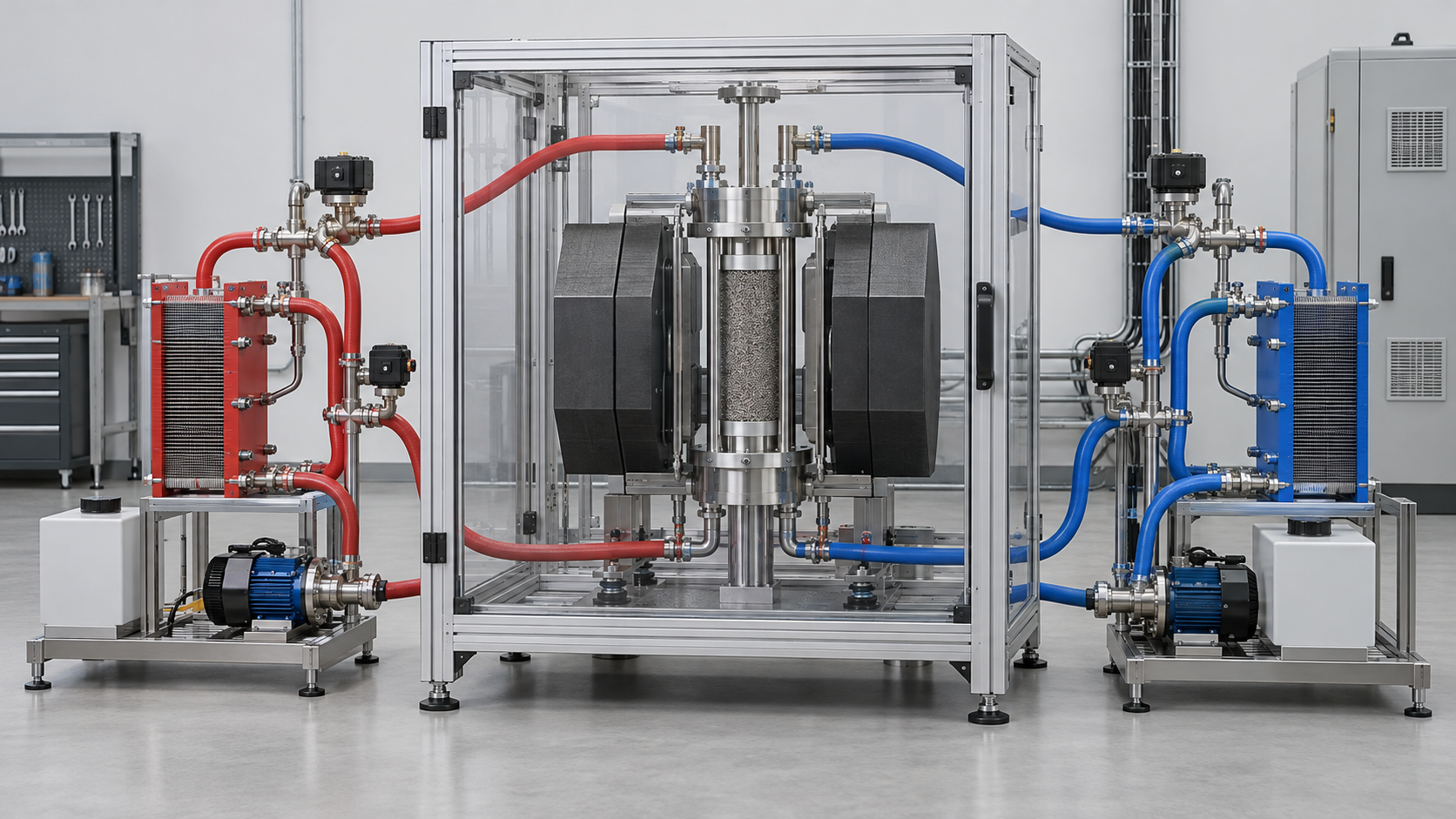
As problem 4 shows, the magnetic material has to be made into a porous structure with fine, straight flow channels so as to maximize contact area with the liquid. But the magnetocaloric effect can drop during processing, and there are reported cases where a material with a large effect in bulk gives only a modest effect once made into a heat exchanger with sub-millimetre channels [Source 2].
The specific examples given by Gutfleisch et al. are as in Chapter 3. La-Fe-Si is brittle and turns to powder, so a resin-bonded plate dilutes the effect. Gd is ductile and easy to work. Mn-Fe-P-Si has low thermal conductivity and the frequency cannot rise. There is also an example in which selective laser melting made a block of La(Fe,Co,Si)13 with wavy channels and an array of thin rods that withstood more than 106 field applications [Source 2]. The processing route (powder, sintering, bonding, additive manufacturing) decides the value of a material as much as the design of its composition does (commentary by this article).
Gutfleisch et al. state that the magnet system is the most expensive part of the machine and also has the largest environmental burden in life-cycle analysis. The field source is assumed to be Nd-Fe-B permanent magnets, with designs aimed at a field change of 0.5–1.2 T [Source 2]. So even if one chooses a refrigerant that uses no rare earths, such as Mn-Fe-P-Si, the machine as a whole still depends on neodymium magnets (which may contain Dy and Tb).
In this sense magnetic refrigeration is continuous with the supply issues in the “Permanent Magnets and Rare Earths” article of this series. At the same time, one reason first-order materials are valued is that they can use a large effect in a small field (1–2 T), which lets the amount of magnet be reduced [Source 2] (commentary by this article).
6. Where prototypes stand — the shift of field source, and the wall of temperature span
The review by Franco et al. organizes prototype room-temperature magnetic refrigerators worldwide. Early machines were driven by superconducting magnets (5–7 T). The 1997 machine of Zimm et al. used a 5 T superconducting magnet and is recorded as running 600 W at a span of 10 K for 18 months. Machines with permanent magnets (mainly Nd-Fe-B) then increased, and the 2001 Astronautics machine ran on a 1.5 T permanent magnetSourced [Sources 3, 4]. The field available from permanent magnets is up to about 1.6 T. This means that the smaller the field, the smaller the ΔTad of the refrigerant, and the more must be built up by AMR (commentary by this article).
Moya et al. estimate the temperature difference (span) a refrigerant needs for a refrigerator as the difference between the compartment temperature and the ambient temperature plus what is lost in two heat exchanges. Our calculation For a 3 °C compartment and 32 °C ambient, 32 − 3 = 29 K, plus a 10 K difference for each of two heat exchanges (20 K in all), gives 49 K. For a freezer (−18 °C), 32 − (−18) = 50 K plus 20 K gives 70 K. These agree with the about 49 K and about 70 K given by Moya et al. [Source 4].
Assumptions and limits: the 10 K difference at the heat exchangers is a setting in the estimate of Moya et al., not a value for real equipment. An ambient temperature of 32 °C is the same as one of the ambient temperatures used in the standard for evaluating refrigerators (Chapter 10).
Here the “reach” of prototypes is set beside the span a refrigerator needs.
- The span falls short: among permanent-magnet machines, the largest reported span is 33 K for the 2013 machine of the University of Victoria (Gd 0.65 kg, 1.6 T, 0.8 Hz), with a cooling power of 50 W at that time. It does not reach the 49 K a refrigerator needs [Source 3]
- Cooling power and span trade off: the machine with a 1.5 T permanent magnet and Gd taken up by Moya et al. delivers 51 W at 18 K, falling to 9 W at 40 K [Source 4]. The machines with larger cooling power tend to have smaller spans (our reading)
- Scaling up raised cooling power: the 2022 prototype of Masche et al. (DTU, Gd 3.83 kg, 1.44 T) reports over 800 W at COP of 4 or more (at a span above 10 K) [Source 5]. A 2023 report gives 452 W, COP 3.2 and a second-law efficiency of 15.5% at a span of 14 K; at part load (245 W) COP was 6.2 and the efficiency 29.7% [Source 6]
- Where efficiency stands: Moya et al. summarize that the most-cited prototype reached about 40% of Carnot at a span of 10 K and about 20% at 20 K, whereas vapour-compression refrigerators reach up to about 60% [Source 4]
The ΔTad of Gd is about 2.5 K per tesla (the table in Chapter 3). Our calculation If it is assumed to grow linearly up to 1.6 T, it comes to about 2.5 × 1.6 = about 4 K. The 33 K span of Victoria is about 8 times this (33 ÷ 4), and the 49 K a refrigerator needs is about 12 times (49 ÷ 4). In other words, the regenerator does the work of building up the temperature change of one material cycle by a factor of 8 to 12.
Assumptions and limits: this is the crude assumption that ΔTad is linear in field; real Gd differs with temperature and field. It is an estimate, not a measured ΔTad at 1.6 T. Because the span is compared with the maximum of a prototype (including conditions close to no load), it is not the amplification in actual operation.
Masche et al. report COP 3.2 and a second-law efficiency of 15.5% at a span of 14 K, and COP 6.2 and 29.7% at part load [Source 6]. Second-law efficiency is COP divided by Carnot COP, so Our calculation the Carnot COP is 3.2 ÷ 0.155 = about 20.6 and 6.2 ÷ 0.297 = about 20.9, nearly the same. Since Carnot COP = Tc / (Th − Tc), a span of 14 K reads as Tc of about 288–293 K (15–20 °C).
Assumptions and limits: this is a back-calculation assuming the two operating points have the same temperature conditions (a 14 K span); the paper does not state the temperatures explicitly. COP depends on cooling power and electrical power, and whether losses of auxiliaries (pumps, motors) are included may be defined differently from paper to paper.
At CES 2015 in January 2015, BASF, Haier and Astronautics announced a “proof-of-concept wine cooler” cooled by a magnetocaloric heat pump. The announcement states that it uses a class of materials based on manganese and iron (developed by BASF and Delft University of Technology), that “theoretical studies” show magnetocaloric refrigeration systems can be up to 35% more energy-efficient than vapour compression, and that Haier plans to introduce the technology to the market within the next couple of yearsNot yet confirmed [Source 9]. This is a company announcement, a theoretical claim and a plan. In this article’s research no commercial product could be confirmed.
Reports of prototypes vary from machine to machine in cooling power, span, COP, field, frequency and the mass of refrigerant. Setting “800 W” beside “33 K” does not say which is better. To compare, one must look at COP or second-law efficiency after matching span, cooling power, field and mass of refrigerant. Cooling power per mass of refrigerant is also useful when evaluating a material (commentary by this article).
Gutfleisch et al. likewise list, as goals for magnetic refrigerators, a low-cost refrigerant, an inexpensive magnet system, valves above 10 Hz, and heat transfer in 50–20 milliseconds reaching 80–90% of theoretical efficiency, which shows that improving one material is not enough [Source 2].
7. Comparison with solid-state cooling — on equal terms
The magnetocaloric effect is one kind of solid-state cooling (cooling that uses no compressor and no refrigerant gas). Thermoelectric (Peltier), electrocaloric and elastocaloric cooling are its relatives, and all of them change the temperature or entropy of a solid with an external field (electric field, stress, magnetic field). In their review comparing these approaches, Wang et al. show that because the type of external field differs between approaches, a simple comparison on one yardstick is not possibleSourced [Source 8]. The table below juxtaposes values stated in the primary literature and is not a ranking.
| Approach | External field | Reported ΔTad (conditions) | Features and issues (as stated in the source) |
|---|---|---|---|
| Magnetocaloric (Gd) | Magnetic field | ΔT 13 K at 294 K and 5 T (ΔS 11 J/(kg·K)) | Permanent magnets as field source give up to about 1.6 T. Mn-Fe-P-Si (Mn1.24Fe0.71P0.46Si0.54) gives 3.0 K at 1 T [4] |
| Electrocaloric (bulk ceramic) | Electric field | PbSc0.5Ta0.5O3: 1.8 K at 25 kV/cm | Values for bulk ceramics are small [4] |
| Electrocaloric (P(VDF-TrFE)-based thin films) | Electric field | 12–21 K at 1,200–3,000 kV/cm | Values at very high fields, for thin-film samples [4] |
| Elastocaloric (NiTi) | Stress | 17–28 K at 0.65–0.9 GPa | Latent heat is 10–15 J/g (equivalent to 20–30 K of ΔTad) [4, 8] |
| Thermoelectric (Peltier) | Electric current | Module maximum span 70–80 K; operated at 30–40 K and tens of W | The maximum span is large, but actual operation is reported in the range of 30–40 K and tens of W [8] |
All Sourced (Moya et al. [Source 4], Wang et al. [Source 8]). The units of external field differ (T, kV/cm, GPa), as do the sample form (bulk, thin film) and the measurement temperature. This does not show a ranking of merit or efficiency.
Wang et al. also organize how far regeneration (a mechanism, like AMR, in which the material itself stores a temperature gradient) can widen the span: about twofold for elastocaloric and more than fivefold for electrocaloric [Source 8]. Read together with the account so far, every solid-state approach shares the feature of making up for a small ΔTad through regeneration, and in each, besides the material, the mechanism that supplies the external field (magnets, high voltage, a stress-applying mechanism) decides the size and cost of the machine (commentary by this article).
8. Resources and supply
The resource issue for magnetic refrigeration splits into refrigerant and field source. Among refrigerants, the benchmark Gd is included in Announcement No. 18 of 2025 of China’s Ministry of Commerce (4 April 2025, in force from the date of promulgation), which covers metals, alloys, oxides and compounds of seven elements: Sm, Gd, Tb, Dy, Lu, Sc and YSourced [Source 11]. No. 18 is in force and is not among those listed in the later suspension by Announcement No. 70 [Source 13].
- Ho: Announcement No. 57 of 2025 (promulgated 9 October 2025) lists, together with permanent-magnet and magnetostrictive materials of Ho, magnetic refrigeration materials containing holmium (the original wording is that of a category of Ho-containing magnetic refrigeration materials). Under Announcement No. 70 (7 November 2025) it is suspended until 10 November 2026 [Sources 12, 13]. What happens after the deadline is Not yet confirmed (could not be confirmed)
- La, Fe, Mn, Si, P: the main elements of La(Fe,Si)13 and Mn-Fe-P-Si systems are not in the lists of seven and five elements in Announcements No. 18 and No. 57 as checked in this article. This article does not, however, judge which category an individual alloy or part falls under
- Field source: the magnet system is assumed to be Nd-Fe-B, and Nd-Fe-B magnets containing Tb or Dy are covered by No. 18. The supply issues treated in the “Permanent Magnets and Rare Earths” article extend directly to magnetic refrigerators [Sources 1, 2]
In other words, even if the refrigerant is changed from Gd to Mn-Fe-P-Si or La-Fe-Si, the dependence on rare-earth magnets for the field source remains (view 4). Rare-earth prices and market forecasts are not covered in this article.
9. Limits, and what could not be confirmed
(1) How to read the values
The values scaled to 1 T in Chapter 3 are approximations converted linearly from literature values by Gutfleisch et al., and mix sample forms (bulk, powder) and measurement methods (direct, indirect). The span, cooling power and COP of prototypes are reported maxima or values at an operating point, and are not matched in conditions.
(2) What could not be confirmed
No standard that directly defines measurement of the magnetocaloric effect (ΔS, ΔTad) could be confirmed. Commercial magnetic refrigerators and their performance, and the outcome of the plans for commercialization stated by BASF, Haier and Astronautics in 2015, have not been confirmed. Neither has the treatment after the deadline of Announcement No. 70 (10 November 2026). Values for the latest prototypes of the solid-state approaches (real elastocaloric and electrocaloric machines) are within the scope of the review by Wang et al. (2023), and later updates have not been checked.
(3) Out of scope
Cooling to very low temperatures by adiabatic demagnetization, magnetic refrigeration for hydrogen liquefaction, details of the phases of Gd5(Si,Ge)4, thermomagnetic power generation, and prices and price forecasts are not covered. For permanent magnets see the “Permanent Magnets and Rare Earths” article, for magnets that use no rare earths the “Rare-Earth-Free Magnets” article. Thermoelectrics is touched on only as a point of comparison in Chapter 7.
- The magnetocaloric effect gives ΔTad of about 2–4 K at 1 T. To reach the about 49 K a refrigerator needs (about 70 K for a freezer), the regenerator has to build up the effect by about 8 to 12 timesSourced / Our calculation
- In first-order materials, a large ΔS and hysteresis are two sides of one coin. In a model, increasing hysteresis cuts COP by up to halfSourced
- A material becomes performance only once it has a shape. Binding powder with resin dilutes the effect, lowers thermal conductivity and lowers the operating frequencySourced
- Prototypes with permanent magnets have reached a span of up to 33 K (50 W), or 452 W at 14 K. They do not yet reach the 49 K a refrigerator needsSourced
- Commercialization is at the stage of a company plan. The 2015 announcement was a plan, and no commercial product could be confirmedNot yet confirmed
10. How to read evaluations and standards
The “performance” of magnetic refrigeration is measured differently at each level: the material (ΔS, ΔTad, specific heat, transition temperature, hysteresis); the field source (Br, HcJ and (BH)max of the permanent magnet, and the gap field inside the machine); the machine (cooling power, span, COP); and the product (the energy consumption of a refrigerator). Of these, no standard that measures the magnetocaloric effect of a material itself could be confirmed in this article.
| Item evaluated | ISO | IEC / IEEE | JIS | ASTM (number and title only) | What changes the value with measurement conditions |
|---|---|---|---|---|---|
| Measurement of the magnetocaloric effect (ΔSm, ΔTad) | Could not be confirmed | Could not be confirmed (IEEE also) | Could not be confirmed | Could not be confirmed | The indirect method works from isothermal magnetization curves; the direct method measures the temperature change adiabatically. Read papers with the conditions (field, temperature, rate of field change) stated. For direct measurement, a field-change rate of about 3 T/s is reported to be needed, and a slower rate does not keep the error within 2% [10] |
| Specific heat capacity Cp (used to convert to ΔTad) | Could not be confirmed | Could not be confirmed | Could not be confirmed | ASTM E1269-24 “Standard Test Method for Determining Specific Heat Capacity by Differential Scanning Calorimetry” (edition seen: E1269-24) [16] | As the title says, a test method for specific heat capacity by differential scanning calorimetry (DSC). Whether it defines measurement of specific heat in a magnetic field has not been checked in this article |
| Energy consumption of household refrigerators (evaluation of the product) | Could not be confirmed | IEC 62552-3:2015 “Household refrigerating appliances – Characteristics and test methods – Part 3: Energy consumption and volume” (1st edition, 2015-02-13) [14] IEEE: could not be confirmed | JIS C 9801-3:2015 “Household refrigerating appliances – Characteristics and test methods – Part 3: Energy consumption and volume” (title in Japanese; MOD of IEC 62552-3; established 22 June 2015) [15] | Could not be confirmed | The IEC page explains that the energy test now specifies two ambient temperatures (16 °C and 32 °C). It is an evaluation of the whole appliance and does not define evaluation of the refrigerant (the magnetocaloric material) |
| Permanent magnets as the field source (Br, HcJ, (BH)max) | Could not be confirmed | IEC 60404-5:2015 (3rd edition) [17]. IEEE: could not be confirmed | JIS C 2501:2019 “Methods of test for permanent magnet” (MOD of IEC 60404-5:2015) [17] | ASTM A977/A977M “Standard Test Method for Magnetic Properties of High-Coercivity Permanent Magnet Materials Using Hysteresigraphs” (edition seen: A977M-07, reapproved 2013) [18] | The standards measure the material properties of the magnet. The gap field inside the machine (set by the magnetic circuit) is not a quantity they measure. See the “Permanent Magnets and Rare Earths” article for details |
| Performance of magnetic refrigerators (cooling power, span, COP) | Could not be confirmed | Could not be confirmed | Could not be confirmed | Could not be confirmed | No test standard could be confirmed, and the operating point (frequency, flow rate, span, load) differs from paper to paper. COP can change depending on whether the losses of pumps and motors are included (a caution from this article) |
The number, title and edition of the standard in each row are Sourced (checked on the IEC Webstore, JSA preview pages, the BSI Knowledge catalogue page and a technical note from Arnold). The arrangement of the table is editorial work, which counts as Our calculation. For ASTM standards, the ASTM site was not opened; only the number and title confirmed from non-ASTM public sources are given, and no test conditions, procedures or acceptance criteria are written. The texts of standards are paid and were not checked.
Cautions when reading standards
- With no standard for measuring ΔS, comparing papers starts with checking conditions. Check the size of the field, the method (direct or indirect), the sample form and the temperature range, and look at whether ΔTad was measured under cyclic conditions
- The refrigerator standards evaluate a product, not a material. IEC 62552-3 and JIS C 9801-3 decide how to measure a refrigerator’s electricity consumption and volume. This article has not checked any material showing how a magnetic refrigerator would perform in that test, or that it satisfied it
- A standard value for a permanent magnet does not guarantee the field in a machine. Br and HcJ of a magnet are values for the material; the gap field in a machine is set by the magnetic circuit
11. Glossary
- Magnetocaloric effect (MCE)
- The reversible change of a substance’s temperature or entropy with a change of external magnetic field.
- ΔTad (adiabatic temperature change)
- The temperature change when the field is changed adiabatically.
- ΔSm (isothermal entropy change)
- The entropy change when the field is changed isothermally. Corresponds to heat Q = TΔSm.
- Maxwell relation
- A thermodynamic relation that gives ΔS from the temperature dependence of magnetization (the basis of the indirect method).
- Second-order / first-order transition
- A second-order transition is continuous. A first-order transition is discontinuous and brings thermal hysteresis.
- Thermal hysteresis
- The shift of the transition temperature between heating and cooling.
- Tricritical point
- The point where a first-order transition becomes second order.
- AMR (active magnetic regenerator)
- A cycle in which a solid regenerator serves as both magnetic refrigerant and heat store and builds up a temperature gradient.
- Regenerator
- A porous structure that temporarily stores heat. Fluid flows through it.
- Span
- The temperature difference between the hot and cold ends (Th − Tc).
- COP
- Coefficient of performance: cooling power divided by the work put in.
- Second-law efficiency
- COP divided by the Carnot COP for the same temperature conditions.
- Relative cooling power (RCP)
- An index made by integrating ΔS over a temperature range. Said to be easily misleading.
- Solid-state cooling
- A general term for cooling that uses no compressor and no refrigerant gas (thermoelectric, magnetocaloric, electrocaloric, elastocaloric and others).
- Electrocaloric effect
- A temperature change caused by a change of electric field.
- Elastocaloric effect
- A temperature change caused by a change of stress. Reported in the phase transformation of NiTi.
12. References (primary sources)
- Sandeman K. G. “Magnetocaloric materials: The search for new systems”, Scripta Mater. 67, 566–571 (2012), DOI 10.1016/j.scriptamat.2012.02.045 (preprint arXiv:1201.3113 checked) — doi.org/10.1016/j.scriptamat.2012.02.045
- Gutfleisch O. et al. “Mastering hysteresis in magnetocaloric materials”, Phil. Trans. R. Soc. A 374, 20150308 (2016), DOI 10.1098/rsta.2015.0308 (preprint arXiv:1604.08487 checked) — doi.org/10.1098/rsta.2015.0308
- Franco V. et al. “Magnetocaloric effect: From materials research to refrigeration devices”, Prog. Mater. Sci. 93, 112–232 (2018), DOI 10.1016/j.pmatsci.2017.10.005 — doi.org/10.1016/j.pmatsci.2017.10.005
- Moya X., Kar-Narayan S., Mathur N. D. “Caloric materials near ferroic phase transitions”, Nat. Mater. 13, 439–450 (2014), DOI 10.1038/nmat3951 — doi.org/10.1038/nmat3951
- Masche M. et al. “Performance assessment of a rotary active magnetic regenerator prototype using gadolinium”, Appl. Therm. Eng. 204, 117947 (2022), DOI 10.1016/j.applthermaleng.2021.117947 — doi.org/10.1016/j.applthermaleng.2021.117947
- Masche M. et al. “Efficient modulation of the magnetocaloric refrigerator capacity”, Int. J. Refrig. 145, 59–67 (2023), DOI 10.1016/j.ijrefrig.2022.10.005 — doi.org/10.1016/j.ijrefrig.2022.10.005
- Masche M., Ianniciello L., Tušek J., Engelbrecht K. “Impact of hysteresis on caloric cooling performance”, Int. J. Refrig. 121, 302–312 (2021), DOI 10.1016/j.ijrefrig.2020.10.012 — doi.org/10.1016/j.ijrefrig.2020.10.012
- Wang Y. et al. “Towards practical elastocaloric cooling”, Commun. Eng. 2, 79 (2023), DOI 10.1038/s44172-023-00129-5 — doi.org/10.1038/s44172-023-00129-5
- BASF (joint announcement with Haier and Astronautics) “Premiere of cutting-edge cooling appliance at CES 2015” (news release, January 2015; a company announcement) — basf.com/…/2015/01/p-15-100
- Ghorai S. et al. “A Setup for Direct Measurement of the Adiabatic Temperature Change in Magnetocaloric Materials”, IEEE Trans. Instrum. Meas. 72 (2023), DOI 10.1109/TIM.2023.3272387 (preprint arXiv:2210.11509 checked) — doi.org/10.1109/TIM.2023.3272387
- Ministry of Commerce and General Administration of Customs, China Announcement No. 18 of 2025, decision on export controls on certain medium and heavy rare-earth items, 4 April 2025 (in Chinese) — mofcom.gov.cn/…/art_5e663d0b…
- Ministry of Commerce and General Administration of Customs, China Announcement No. 57 of 2025, decision on export controls on certain medium and heavy rare-earth items, 9 October 2025 (in Chinese) — mofcom.gov.cn/…/art_9510f263…
- Ministry of Commerce and General Administration of Customs, China Announcement No. 70 of 2025, decision on suspending the implementation of certain export-control announcements, 7 November 2025 (in Chinese) — mofcom.gov.cn/…/art_da147202…
- IEC “IEC 62552-3:2015 Household refrigerating appliances – Characteristics and test methods – Part 3: Energy consumption and volume” (IEC Webstore catalogue page) — webstore.iec.ch/en/publication/21803
- Japanese Standards Association (JSA) “JIS C 9801-3:2015” (preview, in Japanese) — webdesk.jsa.or.jp/preview/pre_jis_c_09801_003…
- BSI Knowledge “ASTM E1269-24” catalogue page (a BSI page, not the ASTM site) — knowledge.bsigroup.com/…/differential-scanning-calorimetry-1
- IEC / Japanese Standards Association (JSA) “IEC 60404-5:2015” (IEC Webstore) and “JIS C 2501:2019” (preview, in Japanese) — webstore.iec.ch/en/publication/22142, webdesk.jsa.or.jp/preview/pre_jis_c_02501…
- Arnold Magnetic Technologies “What is the Magnetic Hysteresis Loop” (TECHNote TN 1501 rev.2015a; its references give the number and title of ASTM A977M-07, reapproved 2013) — arnoldmagnetics.com/…/Tech-Notes_Hysteresis-Loop.pdf
13. Claim-to-source audit
| Claim in the text | Basis | Category |
|---|---|---|
| The definition of the magnetocaloric effect (temperature and entropy change reversibly with field); the relation between ΔS and ΔTad; the values for materials scaled to 1 T (Gd, La-Ca-Sr-Mn-O, La(Fe,Co,Si)13, La(Fe,Mn,Si)13Hx, Mn-Fe-P-Si, Heusler alloys, Gd5(Si,Ge)4, Fe49Rh51) and their features and issues; the values for the polymer-bonded composite (ΔTad 4.9 K, ΔSm 63 mJ/(cm³·K), thermal conductivity about 5 W/(K·m), operating frequency about 1.5 times lower); that RCP is misleading; that a large ΔS is not a sufficient condition; the effects of hysteresis and ways to reduce it; the four problems of AMR; that the magnet system is the most expensive and has the largest environmental burden | Gutfleisch et al. (2016) Reference 2 https://doi.org/10.1098/rsta.2015.0308 | Sourced |
| The integral expressions for ΔS and ΔTad; the guide of at least 1 K of ΔTad in 1 T from permanent magnets; the formula (Msat·T·μ0Hmax / Cp)1/2 for the maximum ΔTad and about 15 K for Fe-Rh; that most materials give 4–7 K at 2 T; that no single figure of merit has been settled | Sandeman (2012) Reference 1 https://doi.org/10.1016/j.scriptamat.2012.02.045 | Sourced |
| Brown 1976 and Steyert 1978; Zimm 1997 (5 T, 600 W at 10 K, 18 months); Astronautics 2001 (1.5 T permanent magnet); the chronology of peak field, field source and span of prototypes (values in Figs. 6 and 7); Victoria 2013 (33 K, 50 W, Gd 0.65 kg, 1.6 T, 0.8 Hz); the description of the AMR cycle (Fig. 4); the use of Nd-Fe-B | Review by Franco et al. (2018) Reference 3 https://doi.org/10.1016/j.pmatsci.2017.10.005 | Sourced |
| The spans needed for a refrigerator and a freezer (about 49 K and about 70 K); ΔS of 11 J/(kg·K) and ΔT of 13 K for Gd at 294 K and 5 T; 3.0 K at 1 T for Mn-Fe-P-Si; the efficiency of the most-cited prototype (about 40% of Carnot at 10 K, about 20% at 20 K, up to about 60% for vapour compression); 51 W (18 K) and 9 W (40 K) for the 1.5 T Gd machine; the values for electrocaloric (1.8 K; 12–21 K) and elastocaloric (17–28 K) | Review by Moya et al. (2014) Reference 4 https://doi.org/10.1038/nmat3951 | Sourced |
| The DTU prototype (Gd 3.83 kg, 1.44 T, over 800 W at COP 4 or more, span above 10 K); the 2023 report (452 W at 14 K, COP 3.2, second-law efficiency 15.5%; part load 245 W with COP 6.2 and 29.7%) | Masche et al. (2022, 2023) Reference 5 https://doi.org/10.1016/j.applthermaleng.2021.117947 Reference 6 https://doi.org/10.1016/j.ijrefrig.2022.10.005 | Sourced |
| That when entropy generation by hysteresis goes from 0.5% to 1%, COP falls by up to 50% (numerical model); the tolerance of materials with small specific heat | Masche et al. (2021) Reference 7 https://doi.org/10.1016/j.ijrefrig.2020.10.012 | Sourced |
| The maximum span of a thermoelectric module of 70–80 K, operation at 30–40 K and tens of W; latent heat of NiTi of 10–15 J/g and its conversion to 20–30 K of ΔTad; widening of span by regeneration (about twofold for elastocaloric, more than fivefold for electrocaloric) | Wang et al. (2023) Reference 8 https://doi.org/10.1038/s44172-023-00129-5 | Sourced |
| The January 2015 announcement of a prototype magnetic-refrigeration wine cooler; materials based on manganese and iron; “up to 35% more energy-efficient according to theoretical studies”; Haier’s plan to introduce to the market within a couple of years. No commercial product could be confirmed | News release by BASF, Haier and Astronautics (company announcement and target) Reference 9 https://www.basf.com/global/en/media/news-releases/2015/01/p-15-100 | Not yet confirmed |
| That direct measurement of ΔTad needs a field-change rate of about 3 T/s (for 2% error) | Ghorai et al. (2023) Reference 10 https://doi.org/10.1109/TIM.2023.3272387 | Sourced |
| Announcement No. 18 of 2025 (seven elements including Gd, in force from the date of promulgation); No. 57 (includes magnetic refrigeration materials of Ho, promulgated 9 October 2025); No. 70 (suspends No. 57 and others until 10 November 2026; No. 18 is not among those listed). The treatment after the deadline could not be confirmed | Announcements of the Ministry of Commerce and General Administration of Customs Reference 11 https://www.mofcom.gov.cn/zcfb/blgg/gg/2025/art/2025/art_5e663d0bfec7452dabd950d0f0e42153.html Reference 12 https://www.mofcom.gov.cn/zcfb/blgg/gg/2025/art/2025/art_9510f263c3c246d8936fbfa684a58ca8.html Reference 13 https://www.mofcom.gov.cn/zcfb/blgg/gg/2025/art/2025/art_da147202d0934ddebe252772e95ed7b3.html | Sourced (after the No. 70 deadline: Not yet confirmed) |
| Standards: IEC 62552-3:2015 (ambient temperatures of 16 °C and 32 °C); JIS C 9801-3:2015 (MOD) | IEC Webstore; JSA preview Reference 14 https://webstore.iec.ch/en/publication/21803 Reference 15 https://webdesk.jsa.or.jp/preview/pre_jis_c_09801_003_000_2015_j_ed10_ch.pdf | Sourced |
| Standard: ASTM E1269-24 (title). The ASTM site was not opened; checked on the BSI catalogue page | BSI Knowledge Reference 16 https://knowledge.bsigroup.com/products/standard-test-method-for-determining-specific-heat-capacity-by-differential-scanning-calorimetry-1 | Sourced |
| Standards: IEC 60404-5:2015, JIS C 2501:2019, ASTM A977M-07 (title only; the ASTM site was not opened, and the title was checked in the references of an Arnold note) | IEC Webstore; JSA preview; Arnold TN 1501 Reference 17 https://webstore.iec.ch/en/publication/22142 Reference 18 https://www.arnoldmagnetics.com/wp-content/uploads/2017/10/FINAL_Tech-Library_Tech-Notes_Hysteresis-Loop.pdf | Sourced |
| The upper limit of ΔTad for Fe-Rh of about 15 K (2 T) and about 11 K (1 T), and its ratios of 86% and 34% to the measurements (12.9 K, 3.6 K); the ratio of volumetric ΔSm of the polymer-bonded material (about 1.6 times Gd, about 0.9 times bulk); the addition of spans for refrigerator and freezer (49 K, 70 K); the amplification of span (about 8 times, about 12 times) against about 4 K of ΔTad of Gd at 1.6 T; the Carnot COP back-calculated from second-law efficiency (about 20.6, about 20.9) and Tc (about 288–293 K) | Our calculation (this article). It assumes Sandeman’s formula (Cp = 6R, Msat = 120 A·m²/kg, T = 300 K), the values of Gutfleisch et al., the settings of the estimate of Moya et al., and the COP and efficiency of Masche et al. It involves a linear approximation and the assumption that two operating points share conditions; these are not measurements or machine performance | Our calculation |
| A standard measuring the magnetocaloric effect, a test standard for magnetic refrigerators, the products and performance of commercial magnetic refrigerators, the outcome of the commercialization plan of BASF and others, the treatment after the deadline of Announcement No. 70, values for the latest solid-state prototypes, and prices and price forecasts | Could not be confirmed in the primary sources accessible within this article’s research, or not covered by the policy of this article, so not stated | Commentary |
| The readings that “a large ΔS is only the entrance”, “hysteresis is the flip side of a large ΔS”, “a material becomes performance only once it has a shape”, “even if the refrigerant is rare-earth-free, the field source is a rare-earth magnet”, and “compare at the same span, load and field” | This article’s arrangement and commentary based on published content. They are not views stated by the companies or institutions | Commentary |
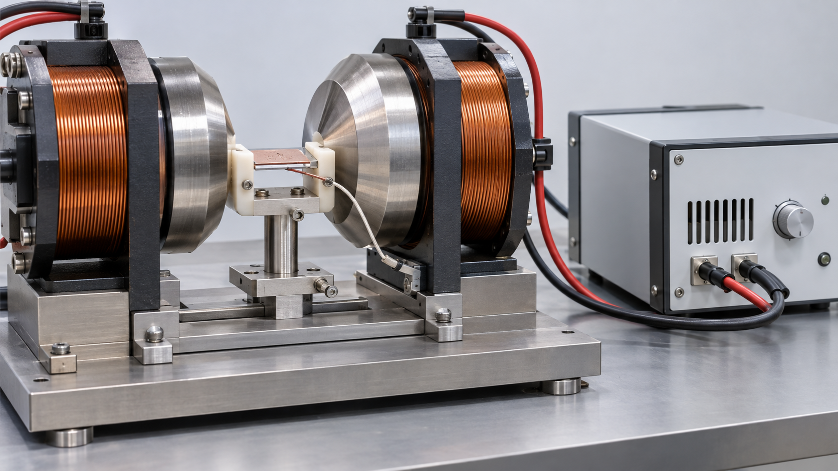
| That Figs. 2 to 4, 6 and 7 are explanatory drawings, not measured figures or real data, and that Figs. 1 and 5 are AI-generated images | Note from this article | Commentary |
Last updated 10 October 2026. Sources are limited to primary material (peer-reviewed papers, a company news release, announcements of China’s Ministry of Commerce, and standards-body catalogue pages). The texts of standards are paid and were not checked. The ASTM International site was not opened, because that body states that AI use of the site is not permitted. Some values are quoted as collected in reviews (Franco et al., Gutfleisch et al., Moya et al.), and the original papers were not checked individually. Values of ΔTad, ΔS, span and cooling power are juxtapositions of reports with different material forms, fields and operating points and do not show which is better. Structural readings and materials-design interpretations are marked as Commentary and kept separate from sourced fact. A standard measuring the magnetocaloric effect, the products and performance of commercial magnetic refrigerators, the outcome of the 2015 commercialization plan, and the treatment after the deadline of Announcement No. 70 could not be confirmed and are not stated here. All figures are explanatory concept graphics. Figs. 2 to 4, 6 and 7 are vector drawings; Figs. 1 and 5 are AI-generated images, and none of them shows a real device, material or product.