TECHNOLOGY EXPLAINER
Inference Optimization and Model Serving
— why "fast", "cheap" and "no waiting" pull against each other, and how serving systems strike a balance
When a trained model is run as a live service, most of the time and cost goes into the stage that writes text one token at a time. That stage is limited less by compute than by how fast memory can be read and how much of it there is, which is why batching, KV-cache management, speculative decoding and prefill/decode disaggregation were developed. This article explains how each technique works and how latency, throughput and cost relate, using papers and official evaluation rules, and builds a feel for the numbers with our own calculations.
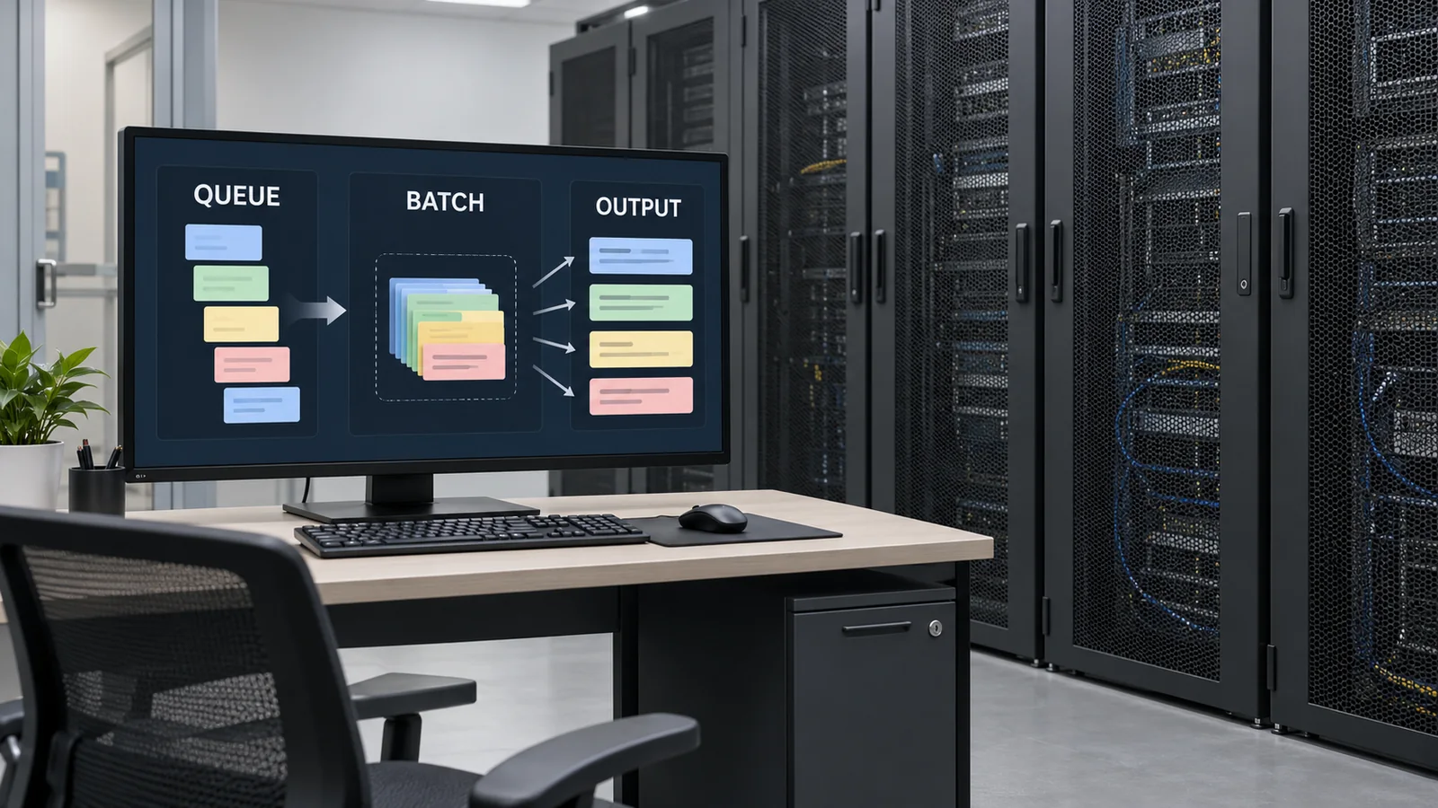
- What inference optimization is (the short version)
- The two stages of inference: prefill and decode
- The KV cache: the in-progress state that occupies memory
- Batching and throughput: more at once is cheaper, but each user waits longer
- Using memory well: PagedAttention, prefix reuse and FlashAttention
- Speculative decoding: a small model drafts, the large model checks in one pass
- Disaggregating prefill and decode, and chunked prefill: avoiding interference
- Reading latency, throughput and cost: the conditions that must accompany a number
- Limits, and what could not be confirmed
- How to read evaluations and standards
- Glossary
- References
- Claim-to-source audit
Sourced = stated in a published source (linked)
Our calculation = a value this article derives from stated assumptions
Not yet confirmed = plans, schedules or proposals not yet confirmed as results
Interpretation and organization are marked as commentary. An inference is shown in bold.
The speeds and speed-up factors here are either values reported by each paper's authors for a specific model, hardware and workload, or values this article estimates with a simple model. Factors from different papers are not lined up to rank them, and no products or companies are compared. Our calculations are idealized upper-bound estimates, not predictions of real-system performance.
1. What inference optimization is (the short version)
- Inference has two stages: "prefill", which reads the whole input at once and is limited by arithmetic, and "decode", which writes the answer one token at a time and is limited by memory reads. Most discussions of speed and cost start from this difference.Sourced[Refs. 1, 13]
- Speed, cost and waiting time cannot all be optimized at once: serving more requests together (a larger batch) improves output and cost per GPU but lengthens the gap between tokens for each user (estimated in Chapter 4).Our calculation
- Memory decides how many users fit at once: the in-progress state of a conversation (the KV cache) grows with every token and occupies GPU memory. How it is stored (for example PagedAttention) and whether the two stages run on separate machines are the heart of practical serving design.Sourced[Refs. 1, 9]
"Tokens per second" and "N times faster" can be compared only when the model, precision, hardware, batch, input and output lengths, software and latency conditions are stated. The MLCommons evaluation rules constrain LLM latency with two numbers, time to first token (TTFT) and time per output token (TPOT), and compare the highest throughput achievable within those limits.Sourced[Ref. 14]
2. The two stages of inference: prefill and decode
A language model writes by predicting the next token, one at a time. Each new token requires a pass through the whole model; Leviathan et al. note that producing K tokens takes K serial runs of the model.Sourced[Ref. 3] The first step, reading the whole input, is different, because all input tokens can be processed in parallel. The Sarathi-Serve paper describes prefill as high-latency but saturating GPU compute, and decode as low-latency but with low compute utilization because each iteration processes only one token per request.Sourced[Ref. 10]
Splitwise describes the same split: prompt computation is compute-intensive and token generation is memory-intensive, each with distinct latency, throughput, memory and power characteristics.Sourced[Ref. 8] For LLM latency, the MLPerf Inference rules define two metrics: TTFT, the latency of the first token, and TPOT, the average interval between generated tokens.Sourced[Ref. 14] Roughly, TTFT corresponds to how long a user waits before anything appears and TPOT to how fast text streams out (this mapping is our commentary).
3. The KV cache: the in-progress state that occupies memory
A Transformer computes attention between each new token and every earlier token. Recomputing the keys and values of past tokens each time would be wasteful, so they are stored and reused: this is the KV cache. The size per token is 2 (key and value) x layers x number of KV heads x head dimension x bytes per element (our summary).
The vLLM paper shows that for OPT-13B in FP16 one token's KV cache is 800 KB (2 x 5,120 x 40 layers x 2 bytes), so a 2,048-token request can need up to 1.6 GB.Sourced[Ref. 1] It also reports, for a 13B model on a 40 GB NVIDIA A100, that about 65% of memory held the weights and close to 30% held the per-request dynamic state, mainly the KV cache.Sourced[Ref. 1] The larger the KV cache, the fewer users can be held at once and the lower the throughput.
Recent models therefore use designs that shrink the KV cache. Grouped-query attention (GQA) of Ainslie et al. uses fewer key/value heads than query heads, aiming for quality close to multi-head attention at speed comparable to multi-query attention.Sourced[Ref. 6] The Llama 3 paper says it uses GQA with 8 key-value heads to improve inference speed and reduce the size of key-value caches during decoding.Sourced[Ref. 7]
Our calculation We use the configuration in the Llama 3 paper's table for the 8B model (32 layers, model dimension 4,096, 32 attention heads, 8 key/value heads, head dimension 4,096 / 32 = 128).Sourced[Ref. 7] BF16 (2 bytes per element) is assumed.
Per token: 2 x 32 x 8 x 128 x 2 = 131,072 bytes (about 0.13 MB). If the same dimensions had 32 KV heads (plain multi-head attention) it would be 524,288 bytes (about 0.52 MB), four times as much.
One user at 2,048 tokens: 131,072 x 2,048 = about 0.27 GB (about 1.07 GB under the no-GQA assumption).
On an 80 GB GPU: the weights in BF16 take 8 billion x 2 = about 16 GB. If 8 GB is set aside for working buffers (an assumed, illustrative value), 80 - 16 - 8 = 56 GB remains for KV cache, enough for 56 / 0.27 = about 208 users at 2,048 tokens (about 52 under the no-GQA assumption).
Assumptions and limits: the parameter count is the nominal "8 billion", and the 8 GB reserve is a placeholder. Block-management overhead, quantization (for example 8-bit KV) and splitting across several GPUs are not modelled. This is a feel for memory sizes, not a prediction of real concurrency.
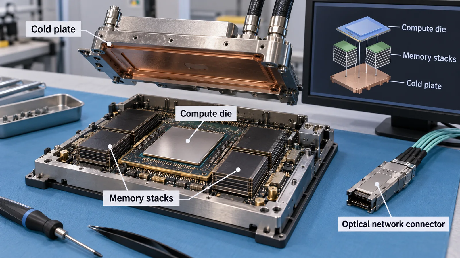
Decode speed is set by how fast the weights and KV cache can be read from memory every token, and the number of users that fit is set by memory capacity (Chapters 3 and 4). A GPU's memory is usually HBM (high bandwidth memory): stacked DRAM dies joined by through-silicon vias and micro-bumps and mounted next to the GPU. The ceiling on inference performance therefore ties directly to the number of HBM stack layers, bandwidth, capacity, and the materials that cool the stack and keep it reliable (encapsulation, thermal interface materials).
Stacking, bonding and heat are covered in this series' explainers on HBM, CoWoS and thermal interface materials. The point here is that software techniques (batching, paged memory, disaggregation) are ways to make the most of memory capacity and bandwidth, which are physical quantities (our commentary).
4. Batching and throughput: more at once is cheaper, but each user waits longer
During decode, all the model weights are read from memory for every token. Whether one user or ten are processed together, the weights are read once. Raising the number of requests processed together (the batch) therefore raises the tokens per second per GPU. The vLLM paper also states that high-throughput serving requires batching sufficiently many requests at a time.Sourced[Ref. 1]
With classic "static batching", everyone waits until the longest response in the batch finishes. Orca (OSDI 2022) proposed iteration-level scheduling, which re-schedules after every single model iteration: requests that finish early can be returned at once and new requests join at the next iteration.Sourced[Ref. 2] This is the idea behind the "continuous batching" used by many serving systems today (that mapping is our commentary).
| Concurrent requests B | Time per step (memory-bound) | Compute-only time | Total tokens/s | Tokens/s per user | Per million tokens (US$) |
|---|---|---|---|---|---|
| 1 | 4.9 ms | 0.0 ms | 206 | 206 | 4.05 |
| 8 | 5.4 ms | 0.1 ms | 1,477 | 185 | 0.56 |
| 32 | 7.3 ms | 0.5 ms | 4,360 | 136 | 0.19 |
| 64 | 9.9 ms | 1.0 ms | 6,462 | 101 | 0.13 |
| 128 | 15.0 ms | 2.1 ms | 8,515 | 67 | 0.10 |
| 208 | 21.4 ms | 3.4 ms | 9,700 | 47 | 0.09 |
All Our calculation. Llama 3 8B (BF16), H100 SXM (3.35 TB/s bandwidth; dense compute taken as half the with-sparsity figure), every user at 2,048 tokens, one GPU, and an illustrative price of US$3 per GPU-hour. Not measured values.
Model: time per step = (16 GB of weights + B x 0.27 GB) / 3.35 TB/s. The H100 SXM memory bandwidth of 3.35 TB/s and 80 GB capacity are NVIDIA's stated values.Sourced[Ref. 13] Every user advances one token per step.
Result: at B = 1 a step takes about 4.9 ms (about 206 tokens/s per user, and the same in total). At B = 208 a step takes about 21.4 ms, so each user gets about 47 tokens/s while the total rises to about 9,700 tokens/s (about 47 times the B = 1 figure). With the illustrative price, cost per million tokens falls from about US$4.05 to about US$0.09.
Compute is left over: in this range the compute-only time is far shorter than the memory time, consistent with Chapter 2's point that decode is set by memory rather than arithmetic. Dense compute is taken as half of the datasheet's with-sparsity figure (about 990 TFLOPS).Sourced[Ref. 13]
Assumptions and limits: real systems lose time to kernel launches, scheduling, communication and imperfect memory use, so actual values are slower. Multi-GPU setups, quantization, mixture-of-experts and prefill time are excluded. The GPU price is a placeholder, not a market price. The calculation only shows the direction: a larger batch lowers each user's speed and raises the total.
5. Using memory well: PagedAttention, prefix reuse and FlashAttention
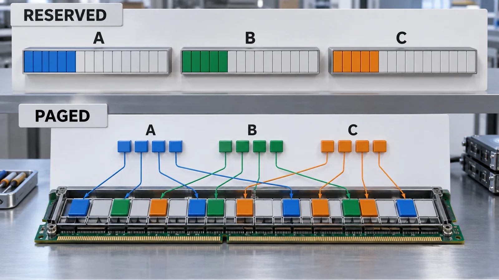
Earlier systems reserved each request's KV cache as one contiguous region sized for the maximum length. Real responses are often much shorter, which wastes reserved-but-unused space (internal fragmentation) and leaves gaps between regions (external fragmentation). In the vLLM paper's measurements, only 20.4% to 38.2% of the KV-cache memory in existing systems held actual token states.Sourced[Ref. 1]
PagedAttention follows operating-system virtual memory and paging: the KV cache is split into fixed-size blocks that can sit in non-contiguous places, linked to their logical order by a block table. Waste is then confined mostly to the last block, and blocks can be shared within and across requests. The vLLM authors report 2x to 4x higher throughput than the state-of-the-art systems FasterTransformer and Orca at the same latency level (values under the authors' own conditions).Sourced[Ref. 1]
View original SVG, values and source annotations
When many requests share the same beginning (a system prompt or a common document), the KV cache for that part can be reused instead of recomputed. The SGLang paper proposes RadixAttention for this and reports up to 6.4x higher throughput on tasks such as multi-turn chat and retrieval-augmented pipelines (under the authors' conditions).Sourced[Ref. 12] Whether reuse pays off depends on how much of the prompt is shared and how much cache memory can be kept (our commentary).
The attention computation itself is also limited by memory traffic. FlashAttention is an IO-aware, exact (not approximate) attention algorithm that uses tiling to reduce reads and writes between the GPU's large HBM and its small, fast on-chip SRAM.Sourced[Ref. 5] Because it reduces memory movement without changing the result, it belongs with "same output, faster" techniques such as speculative decoding in the next chapter (this grouping is our own).
6. Speculative decoding: a small model drafts, the large model checks in one pass
Decode is slow because of weight reads, while arithmetic has headroom (Chapter 4). The idea: a cheap small model (the draft) proposes several tokens ahead, and the large model checks them in parallel, advancing several tokens at once when they are right. Leviathan et al. designed the accept/reject rule so that the output distribution is unchanged and report a 2x to 3x speed-up on T5-XXL,Sourced[Ref. 3] and Chen et al. report 2x to 2.5x on the 70-billion-parameter Chinchilla in a distributed setupSourced[Ref. 4] (both under the authors' conditions).
Leviathan et al. let the acceptance rate α be the average probability that a drafted token is accepted by the large model, c the cost of one draft step relative to one large-model step, and γ the number of tokens drafted per round. They derive the expected tokens per round as (1 - α^(γ+1)) / (1 - α) and the expected wall-time improvement as (1 - α^(γ+1)) / ((1 - α)(γc + 1)), under the simplification that acceptance is independent and equally likely per token.Sourced[Ref. 3]
| Acceptance rate α | γ = 2 | γ = 4 | γ = 8 |
|---|---|---|---|
| 0.4 | 1.42x | 1.37x | 1.19x |
| 0.6 | 1.78x | 1.92x | 1.77x |
| 0.8 | 2.22x | 2.80x | 3.09x |
| 0.9 | 2.46x | 3.41x | 4.38x |
All Our calculation (the formula of Leviathan et al. [Ref. 3] with c = 0.05). The cost ratio c = 0.05 is illustrative; the paper reports c below 0.05 for drafts about two orders of magnitude smaller.
Three cautions. First, the verification step adds arithmetic, so total computation rises; Leviathan et al. frame the method as trading extra arithmetic for lower latency.Sourced[Ref. 3] It helps when decode is stalled on memory rather than arithmetic, and the benefit can shrink when large batches leave little spare compute (this reading follows from the paper's statement about extra operations and is our commentary, not a measurement). Second, the draft can be a separate small model, or the large model's own internal features can predict the next tokens (for example EAGLE), so implementations differ.Sourced[Ref. 19] Third, in evaluation, the MLPerf Inference rules allow speculative decoding only for specific workloads, with the reference prediction head and configuration fixed by the rules.Sourced[Ref. 14]
7. Disaggregating prefill and decode, and chunked prefill: avoiding interference
Mixing prefill and decode on the same GPU lets a long prefill stall the responses of other users who are mid-decode. The DistServe paper points out that existing systems batch both phases together on the same GPUs, causing strong interference and coupling the resource allocation and parallelism plans of the two phases.Sourced[Ref. 9] There are two broad remedies.
- Chunked prefill: Sarathi-Serve splits a prefill into near-equal chunks and builds "stall-free" schedules that add new requests without pausing ongoing decodes. For Mistral-7B on a single A100 the authors report 2.6x the serving capacity (work handled within tail-latency limits) of vLLM (under the authors' conditions).Sourced[Ref. 10]
- Disaggregation: run prefill and decode on separate GPU groups and pass the KV cache between them. Splitwise reports 1.4x higher throughput at 20% lower cost, or 2.35x more throughput at the same cost and power budget;Sourced[Ref. 8] DistServe reports serving up to 7.4x more requests, or meeting a 12.6x tighter latency target, within latency constraintsSourced[Ref. 9] (both under the authors' conditions).
Mooncake is the serving platform of Moonshot AI's Kimi service. It separates prefill and decode clusters and uses the otherwise idle CPU, DRAM and SSD of the GPU cluster as a place to keep KV cache. The authors state that, under real workloads, the design let Kimi handle 75% more requests (the company's own report).Sourced[Ref. 11]
| Method | What it changes | Authors' report (with conditions) | Main cost or condition |
|---|---|---|---|
| Continuous batching (Orca) | Scheduling after every iteration | 36.9x throughput over FasterTransformer at the same latency level on GPT-3 175B [2] | More complex scheduler |
| PagedAttention (vLLM) | How KV is stored (paging) | 2x to 4x throughput at similar latency [1] | Overhead of indirection through block tables |
| Speculative decoding | Several tokens per verification | 2x to 3x on T5-XXL [3]; 2x to 2.5x on Chinchilla 70B [4] | More arithmetic; depends on acceptance rate |
| Chunked prefill (Sarathi-Serve) | Fragments prefill and mixes it in | 2.6x vLLM serving capacity on Mistral-7B, one A100 [10] | Chunking overhead |
| Disaggregation (Splitwise, DistServe) | Prefill and decode on separate GPUs | 1.4x throughput at 20% lower cost [8]; up to 7.4x requests [9] | KV transfer; depends on layout and network |
All Sourced (each paper's authors' reports). Baselines, models, hardware and workloads differ between papers, so the factors in the table cannot be compared with each other to rank the methods.
Splitwise designs its split from the observation that the token-generation phase does not need the latest GPU compute and can run at lower power and cost.Sourced[Ref. 8] If the same work runs on fewer machines with less power, rack heat and incoming power fall. Improvements in inference software therefore connect to the power and cooling problems of data centers (see our explainer on power and cooling for AI data centers).
Conversely, a software speed-up does not necessarily lower energy per token (J/token): filling the GPU with a large batch or adding arithmetic through speculative decoding can cut either way. Energy should be measured under rules such as MLPerf Power (Chapter 10), and speed-up factors alone should not be used to talk about energy (our commentary).
8. Reading latency, throughput and cost: the conditions that must accompany a number
As Chapters 4 to 7 showed, the same system can give numbers that differ by several times depending on conditions. The table lists what to check when you see a claim about speed or cost (our summary).
| Item to check | Why it matters |
|---|---|
| Model and size (total and active parameters) | In mixture-of-experts models the total and the per-token active counts differ. If undisclosed, do not estimate |
| Precision (BF16, FP8, 4-bit, ...) | Changes the bytes of weights and KV, and so speed and concurrency. Check that quality is preserved |
| Hardware, count and interconnect | Memory bandwidth, capacity and GPU-to-GPU communication set the limits |
| Batch / concurrent connections | Total tokens/s and per-user speed trade off (Chapter 4) |
| Input and output lengths | Change prefill cost and KV size; long contexts change the picture a lot |
| Latency conditions (TTFT, TPOT, which percentile) | Is it the maximum throughput within latency limits, or an unconstrained maximum? |
| Software and version | Serving stack and kernel versions can move performance a lot |
| Output quality | Whether the speed-up changed outputs (accuracy target; distribution unchanged?) |
| Power, price and date | Price needs currency, unit, input vs output, date and plan; power needs the scope of measurement |
This list is our own summary of Chapters 4 to 7. Prices change often, so this article quotes no provider's rates.
Jobs where results are not urgent, such as searching internal documents or summarizing experiment logs, give more output per unit cost if run in bulk (offline, large batches). Interactive use with people on the floor is governed by TTFT and TPOT, so it calls for smaller batches that protect latency. Mixing the two on the same equipment makes them affect each other, so each use should have its own latency target (SLO) set at design time (our commentary).
When confidential data cannot leave the company, inference runs on your own GPUs and, as in Chapter 3, GPU memory capacity decides how many people can use it at once. The number of GPUs needed depends on the combination of model size, precision, context length and concurrent users, so a catalogue "tokens per second" figure alone cannot settle it (our commentary).
9. Limits, and what could not be confirmed
- No real measurements are shown: our calculations are idealized estimates that assume memory-bound decode. Individual MLPerf submission results and cross-vendor hardware comparisons are not shown because their settings are not aligned.
- Techniques not covered in depth: quantization details, expert parallelism for MoE, communication costs of tensor and pipeline parallelism, KV-cache quantization and compression, and sliding-window attention (see our explainer on model efficiency).
- Differences between serving stacks: features and version-by-version differences of vLLM (open source under Apache-2.0; the repository was seen to be updated on 14 October 2026),Sourced[Ref. 20] SGLang and other stacks were not verified.
- Prices: API rates change quickly and need an official price page and a date, so none are given. The cost example uses an illustrative US$3 per GPU-hour.
- Standards: no international standard defining LLM inference latency or throughput was found. ISO/IEC 22989 is a terminology standard.
- Prefill tends to be compute-bound and decode memory-bound. That difference is the starting point of most techniques.Sourced
- Larger batches raise the total and lower per-user speed. In our simple estimate, going from B = 1 to B = 208 raised the total about 47-fold while each user got about 23% of the original speed.Our calculation
- Memory management decides concurrency. PagedAttention targets the 20.4% to 38.2% effective KV-memory use seen in earlier systems.Sourced
- Some techniques keep outputs unchanged (speculative decoding) and others change the layout (disaggregation). The factors are condition-specific reports from each paper.Sourced
- MLPerf Inference rules are the main yardstick, but standards cover terminology and no international standard deciding pass or fail on performance was found.
10. How to read evaluations and standards
Inference performance is evaluated by combining four things: (1) latency (TTFT and TPOT), (2) the throughput achievable within latency limits, (3) whether output quality is preserved, and (4) power. The most widely used public framework is MLCommons' MLPerf Inference, which defines server and offline scenarios that imitate user arrivals and sets, per LLM benchmark, TTFT and TPOT limits and an accuracy target.Sourced[Ref. 14] As of 15 October 2026 the MLCommons benchmark page shows MLPerf Inference v6.1,Sourced[Ref. 15] and the 16 September 2026 announcement reports 30 submitting organizations and new tests including an end-to-end RAG benchmark.Sourced[Ref. 15]
| Item | Representative benchmarks and methods (name, source) | Standards and guidance | How to read it |
|---|---|---|---|
| Latency (TTFT, TPOT) | MLPerf Inference rules (rules document, checked 15 Oct 2026). Examples: DeepSeek-R1 Server TTFT/TPOT 2,000 ms/80 ms, Interactive 1,500 ms/15 ms; Llama 2 70B Conversational 2,000 ms/200 ms, Interactive 450 ms/40 ms [14] Sourced | No ISO/IEC or similar standard defining LLM response latency was found. Terminology: ISO/IEC 22989:2022 (AI concepts and terminology) [18] Sourced | Limits differ per benchmark and scenario and are revised between versions. Check the version before using a number |
| Throughput within latency limits | MLPerf Server scenario (Poisson arrivals; the metric is the maximum Poisson arrival rate that meets the latency constraint) and Offline scenario (all samples issued at start) [14] Sourced. In research, DistServe's goodput (rate of requests meeting both TTFT and TPOT constraints) [9] | None found | Offline has no latency constraint and gives a different number from Server. Compare like with like |
| Output quality | MLPerf sets accuracy targets (e.g. Llama 3.1 8B summarization at 99% or 99.9% of the FP32 reference; DeepSeek-R1 at 99% of the FP16 reference) [14] Sourced. Speculative decoding is proven in the paper to leave the distribution unchanged [3] | None found | "99% of reference" refers to that task's metric and does not guarantee quality on other tasks |
| Power and energy | MLPerf Power (Tschand et al., arXiv 2410.12032) describes MLPerf's system power measurement [17] Sourced | None found | Only some submissions include power, and the measurement scope (whole system?) is a condition. Look at it separately from speed-up factors |
| History of the framework itself | Design of MLPerf Inference: Reddi et al. (ISCA 2020) [16] Sourced | Future change: MLCommons says "MLPerf Endpoints", built on an API-centric harness, will replace Inference for the datacenter [15] Not yet confirmed | The benchmark mix changes every round. Avoid comparing numbers across years |
Category tags appear in each cell. The MLPerf latency limits are transcribed from the rules document on GitHub (master as of 15 October 2026) and change between versions. The arrangement of the table is our own.
Three points on how to read these.
- Numbers depend on settings and who measured: MLPerf has submitters measure with their own optimizations, but the rules fix the harness, accuracy targets and even whether speculative decoding is allowed. A factor measured outside such rules is a different thing.
- Benchmarks get replaced: MLPerf Inference changes its models and scenarios by version (for example, v6.1 added an end-to-end RAG test and an edge agentic test). Do not treat an old round's numbers as current.
- Standards mostly cover terminology: within this article's research no international standard setting speed or latency requirements for LLM inference was found. ISO/IEC 22989 covers concepts and terminology and does not decide pass or fail on performance. Performance claims depend on the rules and conditions of public benchmarks.
11. Glossary
- TTFT
- Time to first token: how long until the first token appears.
- TPOT
- Time per output token: the average interval between generated tokens.
- Prefill / decode
- The stage that processes the input at once / the stage that generates one token at a time.
- KV cache
- Stored keys and values of past tokens.
- Batch
- A group of requests processed together.
- Continuous batching
- Letting requests enter and leave after every iteration (proposed by Orca).
- PagedAttention
- Managing the KV cache in fixed-size blocks (vLLM).
- GQA
- Grouped-query attention: fewer key/value heads than query heads.
- Speculative decoding
- Drafting with a small model and verifying in parallel with the large one.
- Acceptance rate α
- Average probability that a drafted token is accepted.
- Goodput
- Rate of requests that meet the latency constraints.
- SLO
- Service level objective: a target for latency and similar measures.
- Memory-bound
- A state where memory traffic rather than arithmetic sets performance.
- HBM
- High bandwidth memory: stacked DRAM mounted next to the GPU.
12. References
- Kwon W. et al. "Efficient Memory Management for Large Language Model Serving with PagedAttention", SOSP '23 (2023), DOI 10.1145/3600006.3613165, arXiv 2309.06180 — arxiv.org/abs/2309.06180
- Yu G.-I. et al. "Orca: A Distributed Serving System for Transformer-Based Generative Models", OSDI '22 (2022) — usenix.org/conference/osdi22/presentation/yu
- Leviathan Y. et al. "Fast Inference from Transformers via Speculative Decoding", ICML 2023, PMLR 202 (2023), arXiv 2211.17192 — proceedings.mlr.press/v202/leviathan23a.html
- Chen C. et al. "Accelerating Large Language Model Decoding with Speculative Sampling", arXiv 2302.01318 (2023) — arxiv.org/abs/2302.01318
- Dao T. et al. "FlashAttention: Fast and Memory-Efficient Exact Attention with IO-Awareness", NeurIPS 2022, arXiv 2205.14135 — arxiv.org/abs/2205.14135
- Ainslie J. et al. "GQA: Training Generalized Multi-Query Transformer Models from Multi-Head Checkpoints", EMNLP 2023, DOI 10.18653/v1/2023.emnlp-main.298, arXiv 2305.13245 — arxiv.org/abs/2305.13245
- Grattafiori A. et al. (Meta) "The Llama 3 Herd of Models", arXiv 2407.21783 (2024) (Table 3: the 8B model has 32 layers, model dimension 4,096, 32 heads and 8 key/value heads) — arxiv.org/abs/2407.21783
- Patel P. et al. "Splitwise: Efficient Generative LLM Inference Using Phase Splitting", ISCA 2024, DOI 10.1109/ISCA59077.2024.00019, arXiv 2311.18677 — arxiv.org/abs/2311.18677
- Zhong Y. et al. "DistServe: Disaggregating Prefill and Decoding for Goodput-optimized Large Language Model Serving", OSDI '24 (2024), arXiv 2401.09670 — usenix.org/conference/osdi24/presentation/zhong-yinmin
- Agrawal A. et al. "Taming Throughput-Latency Tradeoff in LLM Inference with Sarathi-Serve", OSDI '24 (2024), arXiv 2403.02310 — usenix.org/conference/osdi24/presentation/agrawal
- Qin R. et al. (Moonshot AI and others) "Mooncake: A KVCache-centric Disaggregated Architecture for LLM Serving", arXiv 2407.00079 (2024) (the FAST '25 version is titled "Mooncake: Trading More Storage for Less Computation — A KVCache-centric Architecture for Serving LLM Chatbot") — arxiv.org/abs/2407.00079
- Zheng L. et al. "SGLang: Efficient Execution of Structured Language Model Programs", arXiv 2312.07104 (2023) — arxiv.org/abs/2312.07104
- NVIDIA "NVIDIA H100 Tensor Core GPU" (H100 SXM: 80 GB GPU memory, 3.35 TB/s memory bandwidth, Tensor Core figures stated with sparsity, max TDP up to 700 W; checked 15 October 2026) — nvidia.com/en-us/data-center/h100/
- MLCommons "MLPerf Inference Rules" (inference_rules.adoc in the inference_policies repository; master as checked on 15 October 2026. Definitions of TTFT/TPOT, scenarios, accuracy targets and latency limits of the LLM benchmarks, and the speculative-decoding appendix) — github.com/mlcommons/inference_policies/blob/master/infer...
- MLCommons "MLCommons Sets Participation Record with New MLPerf Inference v6.1 Benchmark Results" (announcement of 16 September 2026; syndicated GlobeNewswire page), and the benchmark page https://mlcommons.org/benchmarks/inference-datacenter/ (v6.1 shown; checked 15 October 2026) — financialcontent.com/article/gnwcq-2026-9-16-mlcommons-se...
- Reddi V. J. et al. "MLPerf Inference Benchmark", ISCA 2020, DOI 10.1109/ISCA45697.2020.00045, arXiv 1911.02549 — arxiv.org/abs/1911.02549
- Tschand A. et al. "MLPerf Power: Benchmarking the Energy Efficiency of Machine Learning Systems from Microwatts to Megawatts for Sustainable AI", arXiv 2410.12032 (2024) — arxiv.org/abs/2410.12032
- ISO/IEC "ISO/IEC 22989:2022 Information technology — Artificial intelligence — Artificial intelligence concepts and terminology" (Edition 1, July 2022; JTC 1/SC 42) — iso.org/standard/74296.html
- Li Y. et al. "EAGLE: Speculative Sampling Requires Rethinking Feature Uncertainty", ICML 2024, arXiv 2401.15077 — arxiv.org/abs/2401.15077
- vLLM project GitHub repository vllm-project/vllm (Apache-2.0 license; update seen on 14 October 2026) — github.com/vllm-project/vllm
13. Claim-to-source audit
| Claim in the text | Basis | Category |
|---|---|---|
| OPT-13B KV cache of 800 KB per token (2 x 5,120 x 40 layers x 2 bytes), up to 1.6 GB at 2,048 tokens; about 65% weights and about 30% dynamic state on a 40 GB A100; 20.4% to 38.2% effective KV use in existing systems; the PagedAttention design; 2x to 4x throughput (vs FasterTransformer and Orca at similar latency) | Reference 1 https://arxiv.org/abs/2309.06180 | Sourced |
| Iteration-level scheduling and selective batching (Orca); under static batching finished requests cannot be returned early and new requests wait for the current batch; 36.9x throughput over FasterTransformer at the same latency level on GPT-3 175B | Reference 2 https://www.usenix.org/conference/osdi22/presentation/yu | Sourced |
| Definition of speculative decoding, unchanged output distribution, 2x to 3x on T5-XXL, the formulas in α, c and γ (expected tokens and wall-time improvement), c below 0.05, and the increase in arithmetic operations | Reference 3 https://proceedings.mlr.press/v202/leviathan23a.html | Sourced |
| Speculative sampling gives 2x to 2.5x on Chinchilla 70B in a distributed setup | Reference 4 https://arxiv.org/abs/2302.01318 | Sourced |
| FlashAttention is an IO-aware exact attention that uses tiling to reduce HBM-SRAM traffic | Reference 5 https://arxiv.org/abs/2205.14135 | Sourced |
| GQA uses fewer key/value heads, aiming for MQA-like speed and quality close to multi-head attention | Reference 6 https://arxiv.org/abs/2305.13245 | Sourced |
| Llama 3 8B configuration (32 layers, model dimension 4,096, 32 heads, 8 key/value heads) and the statement that GQA is used to speed up inference and shrink the KV cache | Reference 7 https://arxiv.org/abs/2407.21783 | Sourced |
| Splitwise: the compute-intensive prompt phase and memory-intensive token-generation phase, the split design, 1.4x throughput at 20% lower cost or 2.35x at the same cost and power | Reference 8 https://arxiv.org/abs/2311.18677 | Sourced |
| DistServe: interference when phases share GPUs, TTFT and TPOT requirements, up to 7.4x more requests or a 12.6x tighter SLO (more than 90% of requests within constraints) | Reference 9 https://www.usenix.org/conference/osdi24/presentation/zhong-yinmin | Sourced |
| Sarathi-Serve: character of prefill and decode, chunked prefill and stall-free scheduling, 2.6x vLLM capacity on Mistral-7B on one A100 | Reference 10 https://www.usenix.org/conference/osdi24/presentation/agrawal | Sourced |
| Mooncake: the platform of Kimi, prefill/decode separation, using CPU, DRAM and SSD for KV cache, 75% more requests under real workloads (company's report) | Reference 11 https://arxiv.org/abs/2407.00079 | Sourced |
| SGLang's RadixAttention and up to 6.4x throughput (authors' conditions) | Reference 12 https://arxiv.org/abs/2312.07104 | Sourced |
| H100 SXM memory of 80 GB, bandwidth of 3.35 TB/s, Tensor Core figures stated with sparsity, max TDP up to 700 W | Reference 13 https://www.nvidia.com/en-us/data-center/h100/ | Sourced |
| MLPerf Inference rules: definitions of TTFT and TPOT, Server and Offline scenarios, examples of LLM latency limits and accuracy targets, and speculative decoding allowed only for specific workloads with the reference prediction head and configuration | Reference 14 https://github.com/mlcommons/inference_policies/blob/master/inference_rules.adoc | Sourced |
| MLPerf Inference v6.1 announced 16 September 2026 with 30 submitting organizations, new end-to-end RAG and edge agentic tests, and the statement that MLPerf Endpoints will replace Inference for the datacenter | Reference 15 https://www.financialcontent.com/article/gnwcq-2026-9-16-mlcommons-sets-participation-record-with-new-mlperf-inference-v61-benchmark-results | Not yet confirmed |
| Design and purpose of MLPerf Inference (ISCA 2020) | Reference 16 https://arxiv.org/abs/1911.02549 | Sourced |
| MLPerf Power describes system power measurement | Reference 17 https://arxiv.org/abs/2410.12032 | Sourced |
| ISO/IEC 22989:2022 establishes AI terminology and concepts (Edition 1, July 2022) | Reference 18 https://www.iso.org/standard/74296.html | Sourced |
| EAGLE is a speculative sampling framework that predicts at the feature level | Reference 19 https://arxiv.org/abs/2401.15077 | Sourced |
| vLLM is Apache-2.0 open source and its repository was updated on 14 October 2026 | Reference 20 https://github.com/vllm-project/vllm | Sourced |
| KV cache of Llama 3 8B (131,072 bytes per token), concurrency on an 80 GB GPU, the batch-vs-speed table (from 4.9 ms, about 9,700 tokens/s, etc.), the speculative-decoding improvement table and the cost example (US$3 per GPU-hour) | Our calculation. Idealized estimates assuming memory-bound decode; the 8 GB reserve, US$3 per GPU-hour and c = 0.05 are assumed values. Not a prediction for real systems | Our calculation |
| Real measurements, providers' prices, any international standard defining LLM inference latency, and comparisons of individual MLPerf submissions | Not confirmed within this article's research (or not shown because settings are not aligned); this article's note | Commentary |
| Readings such as "the KV cache is another way of saying HBM capacity and bandwidth", "energy per token drives cooling and power", and thinking about batch in a plant; the mapping of continuous batching to Orca; the mapping of TTFT/TPOT to user experience | This article's organization and commentary based on published material, not views stated by the organizations | Commentary |
Last updated: 15 October 2026. Sources are limited to primary material (peer-reviewed and conference papers, MLCommons rules and announcements, an NVIDIA datasheet, and the ISO page). Real measurements, providers' prices and any international standard defining LLM inference latency could not be confirmed and are not given. The factors are condition-specific reports by each paper's authors, and our calculations are idealized estimates. Figures 2, 5 and 7 are vector drawings; Figures 3, 4 and 6 include our calculations; Figures 1 and 8 are AI-image placeholders only.