TECHNOLOGY EXPLAINER
NISQ and Hybrid Quantum-Classical Computing
How noisy quantum computers share the work with classical ones
Today's quantum computers cannot yet correct the errors that occur during a computation. Hybrid computing is one idea for making them useful anyway: give the quantum computer only short circuits, and let a classical computer do the tuning. This article first explains "NISQ" with the arrow picture, then runs the two best-known methods (VQE and QAOA) on tiny examples. The second half explains, with conditions stated honestly, why they struggle (noise, barren plateaus, the number of measurements) and what error suppression and error mitigation can and cannot do.
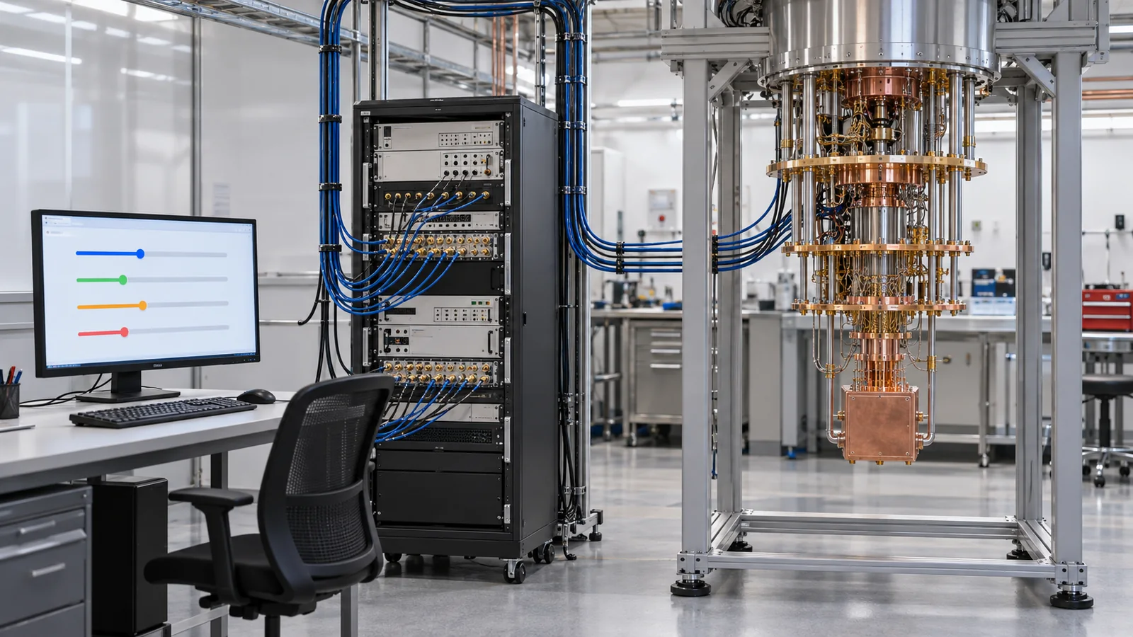
- The short version, what to know first, and where this fits in the series
- Why errors matter: small slips in the arrow add up
- What NISQ means: noisy and intermediate-scale
- Hybrid computing: how quantum and classical machines share the work
- VQE: searching for the lowest energy of a molecule
- QAOA: attacking combinatorial optimization with a quantum circuit
- Why it is hard: noise, barren plateaus and the number of measurements
- Error suppression, mitigation and correction: three different remedies
- A real experiment: IBM's 127-qubit run and what followed
- Limits, what we could not confirm, and a summary
- How to read evaluations and standards
- Glossary
- References
- Claim-to-source audit
Sourced = stated in a published source (linked)
Our calculation = a value computed in this article from the stated assumptions
Not yet confirmed = plans, targets, drafts, work in progress, outlooks: not settled
Our own reading for materials engineers is marked as commentary. Inference is shown in bold. Company announcements are labelled as company claims.
1. The short version, what to know first, and where this fits in the series
- NISQ stands for Noisy Intermediate-Scale Quantum. It describes quantum computers with tens to hundreds of qubits that do not yet have error correction. Preskill proposed the term in 2018 Sourced[Refs. 1, 2]
- Because errors build up, long circuits fall apart. So the quantum computer runs only short circuits and a classical computer tunes the knobs. The best-known examples are VQE (energies of molecules) and QAOA (combinatorial optimization) Sourced[Ref. 3]
- There are three walls: noise, barren plateaus (the learning signal vanishes) and the number of measurements. Error suppression and mitigation get past some of them, but theory shows the cost rises exponentially as circuits get deeper Sourced[Refs. 15, 16]
The basics (qubits, superposition, measurement) are explained in our explainers "Quantum Computing Fundamentals" and "Quantum Gates and Quantum Circuits". This article is readable on its own: it recaps what is needed. No prior knowledge is required.
Recap: the state of a qubit is drawn as an arrow from the centre of a sphere to its surface (north pole = 0, south pole = 1, in between = a superposition of 0 and 1). A gate rotates the arrow. A measurement looks at the arrow and settles on 0 or 1, with probabilities set by the tilt of the arrow. After measuring, the original arrow cannot be recovered.
A good reading order is: Quantum Computing Fundamentals → Quantum Gates and Quantum Circuits → Quantum Algorithms → this article → How to Read Claims of Quantum Advantage → Quantum Error Correction and the Surface Code. The question "could classical computers reproduce the experiments?" is covered in the advantage explainer; VQE for molecules in the quantum chemistry explainer; and QAOA's relative in the quantum annealing explainer.
2. Why errors matter: small slips in the arrow add up
The arrow of a qubit is fragile. When a gate rotates it, the arrow may turn slightly too far or not far enough. Heat and electromagnetic noise from the surroundings can make the arrow wobble (this is called decoherence). Measurement can also be misread. One slip is small, but after hundreds of gates the slips add up.
Let us estimate how fast this happens with the simplest possible formula. Suppose each gate fails with probability ε. Then the probability that all N gates succeed is (1−ε)N.
- Even with a gate error of 0.1% (one in a thousand), stacking 1,000 gates leaves only about a 37% chance that every gate works (0.999^1000 ≈ 0.368) Our calculation
- With a 1% error, 1,000 gates leave about 0.004% (0.99^1000 ≈ 4×10^-5). Cutting the error by ten lets circuits be about ten times longer (N for 50% success: about 69, 693, 6,931) Our calculation
- A real example: one superconducting device reports a two-qubit gate fidelity of 99.62% (Zuchongzhi 3.0, as stated in the abstract) Sourced[Ref. 23]. The error is 0.38%, so success drops to 50% after about 182 gates (ln 0.5 ÷ ln 0.9962 ≈ 182) Our calculation. See the paper for how the figure was measured (average or best, over how many pairs).
A fidelity of 99.62% says how close an operation is to the ideal one; the "error" is what remains (100% − 99.62% = 0.38%). Our explainer on coherence and fidelity covers how it is measured (randomized benchmarking and so on). For this article, remember: the higher the fidelity, the more gates you can stack.
3. What NISQ means: noisy and intermediate-scale
Preskill proposed the term NISQ in a 2018 paper. It says quantum computers with 50 to 100 qubits may be able to perform tasks beyond classical computers, while noise in the gates limits the size of the circuits that can be run Sourced[Ref. 1]. A later review describes NISQ machines as made of hundreds of noisy qubits that are not error-corrected and can perform imperfect operations only within a limited coherence time Sourced[Ref. 2].
| Word | Meaning | Why it matters here |
|---|---|---|
| Noisy | Gates, measurements and idle time all have errors, and none are corrected | Circuits cannot be long (Fig. 2) |
| Intermediate-Scale | Too big to reproduce exactly on classical computers, yet too small for full error correction | The qubit count alone does not set performance; read it together with error rates |
A summary of the definitions in Preskill and in the review (Refs. 1, 2). The boundary of "intermediate scale" shifts with time (our commentary).
A note on example 2 in Fig. 3. Google reported that in two surface-code memories (distance 7 and distance 5), each increase of the code distance by 2 reduced the logical error rate by a factor of Λ = 2.14 ± 0.02, and that the 101-qubit distance-7 code had 0.143% error per cycle Sourced[Ref. 22]. It shows errors being corrected as the code grows, and marks the doorstep of work beyond the NISQ frame. Our explainer on the surface code covers it in detail.
Preskill's 2018 paper mentions "50 to 100 qubits", but what defines NISQ is not the number of qubits; it is that the machine has errors and does not correct them. A later review says NISQ computers already reach hundreds of qubits Sourced[Refs. 1, 2]. The right reading: adding qubits does not leave NISQ if there is no error correction. Judge the stage of a machine by whether it corrects errors, and by its error rates and circuit length.
4. Hybrid computing: how quantum and classical machines share the work
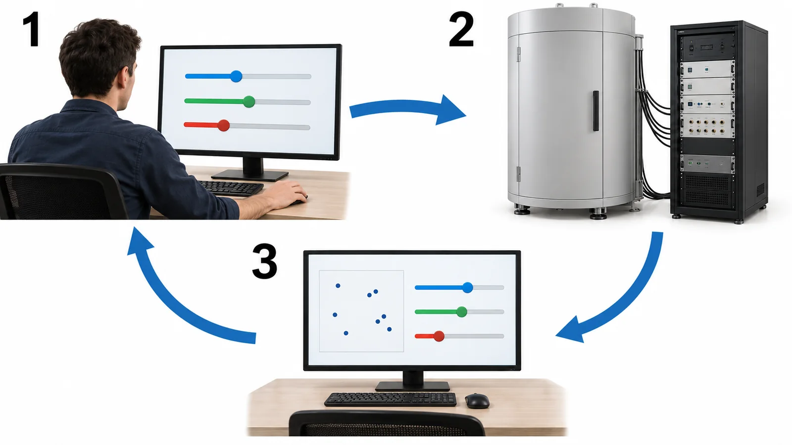
How can a quantum computer that can only run short circuits do useful work? The idea is to give the quantum computer only what it does best and let the classical computer do the rest. Methods of this shape are called variational quantum algorithms (VQAs) Sourced[Ref. 3].
Picture turning the tuning knob of a radio to find the clearest station. The person turning the knob is the classical computer; the radio itself is the quantum computer. Set the knob (θ), listen (the measurement result), turn it a little, and repeat.
View original SVG, values and sources
Original SVG reference: Concept diagram (vector drawing). The loop of a variational quantum algorithm. A classical computer sets the circuit knobs θ, the quantum computer runs the circuit and measures, and the classical computer turns the results into a "cost" and updates θ.
Where the analogy breaks: a radio has one knob, but a quantum circuit has anywhere from a few to thousands. And a radio gives you its sound at once, whereas a quantum circuit gives a different 0 or 1 each time you measure, so the same circuit must be run thousands of times and averaged (one run is called a "shot").
Expectation value: the average of the shot results. For example, if 0 appears 70 times and 1 appears 30 times, counting "0 = +1, 1 = −1" gives (70 − 30) ÷ 100 = 0.4. The "cost" in VQE and similar methods is built from such averages.
| Role | Classical computer | Quantum computer |
|---|---|---|
| Good at | Tuning the knobs (optimization), averaging, post-processing, the calculations behind error mitigation | Preparing and measuring quantum states (complicated correlations between qubits) that are hard to handle classically |
| Weak at | Cannot store the whole state as qubits grow (the state grows exponentially) | Long circuits (errors accumulate), and the shot-to-shot scatter of results |
| Per loop | Send θ / receive results and update θ | Build the circuit for θ, run thousands of shots and return the outcomes |
The division of roles is this article's commentary on the general structure of VQAs (Ref. 3).
5. VQE: searching for the lowest energy of a molecule
VQE (Variational Quantum Eigensolver) searches for the lowest energy of a system (the ground-state energy). The properties of molecules and materials are set by electron energies, so VQE is an entry point to chemistry and materials calculations. In 2014, Peruzzo et al. reported computing the ground-state energy of HeH⁺ to within chemical accuracy (about 1.6 millihartree) on a small photonic quantum processor Sourced[Ref. 4].
(1) The variational principle: no arrow can give an energy below the true bottom
VQE rests on the variational principle. In quantum mechanics, whatever state you prepare, the average energy you measure is at or above the true lowest energy. So if you adjust the knob θ to lower the energy step by step, you approach the true minimum. Since you cannot punch through the floor from above, simply keep going down.
Let us run the smallest possible example. Take one qubit and a simple energy (H = Z): add +1 if you measure 0 and −1 if you measure 1. If the arrow is tilted by an angle θ from the north pole, the probability of 0 is cos²(θ/2), so the average energy is E(θ) = cos θ. It is +1 at θ = 0° (north pole), 0 at θ = 90°, and −1 at θ = 180° (south pole). The minimum is at θ = 180°.
In practice, measuring near θ = 90° with 100 shots gives an average that scatters by about ±0.10 (standard error = √((1−cos²θ)/100) = 0.10) Our calculation. The classical computer watches these noisy values, judges that "a larger θ seems to lower the energy", and moves the knob.
(2) What grows for a real molecule
For a molecule, the number of qubits grows in proportion to the number of orbitals, and the energy expression (the Hamiltonian) becomes a sum of many terms (Pauli terms). A review states that for Gaussian molecular orbital bases the number of terms grows roughly as the fourth power of the number of orbitals (O(M⁴)) Sourced[Ref. 7]. Each term needs its own measurements, so the number of measurements becomes a heavy burden (chapter 7).
| Experiment | Device and scale | What was computed | Reading notes |
|---|---|---|---|
| Peruzzo et al. (2014) | Small photonic quantum processor | Ground-state energy of HeH⁺ (within chemical accuracy) | A tiny two-electron molecule that classical computers solve exactly |
| Kandala et al. (2017) | Superconducting qubits, up to six qubits, over a hundred Pauli terms | Ground-state energies of H₂, LiH and BeH₂, and a quantum magnetism problem | Agreed with numerical simulation including device noise. Not a "beat classical" experiment |
Summary based on the abstracts of Peruzzo et al. (Ref. 4) and Kandala et al. (Ref. 5). Scales are as stated in the papers; comparison with classical computation was not their aim.
The variational principle guarantees that the energy measured on an ideal, noise-free state is never below the floor. On real devices the guarantee does not work as hoped, for two reasons: (1) noise corrupts the state and the search stalls far above the floor; (2) statistical error in the measurements and post-processing for error mitigation can push an estimate below the floor (our commentary). The right reading: a VQE output is a rough upper bound from the states tried, not necessarily the true ground-state energy.
6. QAOA: attacking combinatorial optimization with a quantum circuit
QAOA (Quantum Approximate Optimization Algorithm) was proposed by Farhi et al. in 2014 for problems that ask for the best choice among many combinations (combinatorial optimization) Sourced[Ref. 6]. Take the Max-Cut problem as an example: colour the points in two colours so that the number of links joining points of different colours is as large as possible.
With only five points, checking all 2⁵ = 32 colourings reveals the answer (5 links) Our calculation. With 100 points there are 2^100 ≈ 1.3×10^30 colourings, far too many to check. QAOA uses a quantum circuit to make 0/1 strings in which good colourings are more likely to appear, then measures them. The knobs (γ and β) are tuned by a classical computer.
The paper by Farhi et al. showed that for p = 1 on 3-regular graphs (every point has three links), a cut at least 0.6924 times the optimum is always found Sourced[Ref. 6]. This is a lower-bound guarantee ("at worst this good"); it does not mean the method is better than classical algorithms (our commentary). QAOA is a gate-model method whose idea is close to quantum annealing (see our explainer on quantum annealing).
7. Why it is hard: noise, barren plateaus and the number of measurements
(1) Noise: deeper circuits drift toward "nothing in it"
With noise, the deeper the circuit, the more its output drifts toward random results that carry no information. Stilck França and García-Patrón built a framework for comparing classical and quantum algorithms on noisy devices and found that substantial quantum advantages are unlikely for classical optimization unless noise rates fall by orders of magnitude or the problem's topology matches the device Sourced[Ref. 12]. Wang et al. proved that noise itself creates barren plateaus: under local Pauli noise, if the circuit depth grows linearly with the number of qubits n, the gradient vanishes exponentially in n Sourced[Ref. 10].
(2) Barren plateaus: the hint about which way to go disappears
When tuning θ, the classical computer decides which way to move from the slope (gradient) of the energy. But when a circuit is close to random, the landscape can be a wide plain with almost no slope. McClean et al. showed that for a wide class of circuits the probability that the gradient is non-zero shrinks exponentially with the number of qubits, and named this the barren plateau Sourced[Ref. 8]. It is like searching for a valley bottom in fog when the ground is flat everywhere and you cannot tell which way is down.
However, it does not happen for every circuit. Cerezo et al. showed that a cost function that looks at all qubits causes barren plateaus even in shallow circuits, whereas one that looks at only a few qubits gives at worst a polynomially vanishing gradient for depths up to O(log n) Sourced[Ref. 9]. The same group later argued, with case-by-case evidence, that circuits structured to avoid barren plateaus can often also be handled efficiently by classical computers Sourced[Ref. 11]. So there is a tension: the easier a circuit is to train, the less a quantum computer may be needed for it.
It means shrinking like "halving with every extra qubit": about one in a thousand at 10 qubits, one in a million at 20, and one in a trillion at 40 (the illustration in Fig. 7, 2⁻ⁿ) Our calculation. Not "a little worse as the number grows", but "suddenly hopeless as the number grows".
(3) Number of measurements: ten times the precision needs a hundred times the shots
The statistical error in an expectation value falls in proportion to the inverse square root of the number of shots M (standard error = σ ÷ √M, where σ is the scatter of single outcomes). Google's experimental paper likewise states that the uncertainty of XEB is 1/√(number of samples) Sourced[Ref. 21]. For molecules there are many terms, each measured separately, so the required number of shots balloons.
| Target precision (standard error) | Shots needed (rough worst case, σ = 1) | Reading |
|---|---|---|
| 0.1 | 100 | About 100 shots, as in Fig. 5 |
| 0.01 | 10,000 | Ten times the precision means a hundred times the shots |
| 0.001 | 1,000,000 | Roughly what one term needs for precision near chemical accuracy (0.0016) |
M = (σ ÷ precision)², from standard error = σ ÷ √M. Our calculation. σ = 1 is a rough worst case; the real σ depends on the problem.
As a result, one VQE run amounts to "thousands to millions of shots × tens to thousands of terms × the number of knob adjustments". This takes up a large part of the machine time and cost (our commentary).
The IBM paper by Kim et al. gives, as a reason why the noise model changes over time, that qubits interact with fluctuating microscopic defects (two-level systems, TLS) Sourced[Ref. 18]. For the same device (the 127-qubit Eagle), the median coherence times are reported as T₁ = 288 µs and T₂ = 127 µs Sourced[Ref. 18] (values for superconducting qubits; do not rank them against devices of other types).
Error mitigation fixes errors in software, but as chapter 8 shows, the cost rises exponentially with circuit depth. So improving materials and interfaces (oxide films, substrates, wiring) to lower gate errors is the surest way to lower the cost of mitigation. From a materials standpoint, "qubit quality = size of errors" is also a question of the kind and number of defects and the cleanliness of interfaces (our commentary; see our explainers on superconducting qubits and on materials and fabrication).
8. Error suppression, mitigation and correction: three different remedies
Remedies for errors fall into three groups by when and what they do. Error suppression makes errors less likely while the circuit runs. For example, dynamical decoupling applies short pulses while a qubit waits, cancelling the effect of fluctuations from the surroundings. Ezzell et al. compared 60 pulse sequences on three IBM devices and describe dynamical decoupling as the simplest and least resource-intensive error-suppression strategy Sourced[Ref. 17].
Error mitigation does not fix errors; it corrects the averages of many measurements. A review positions it as the way to soften, rather than completely remove, errors on NISQ-era machines Sourced[Ref. 14]. There are two representative methods Sourced[Ref. 13].
- Zero-noise extrapolation (ZNE): deliberately raise the noise (1x, 2x, 3x), measure, and extrapolate to the value at "zero noise". See Fig. 9 for an example.
- Probabilistic error cancellation (PEC): mix in operations that undo the noise at random, so that on average the noise cancels. The needed number of shots grows rapidly with the number of gates.
In ZNE the answer depends on how you extrapolate, and the scatter in the measurements is amplified by the extrapolation (Fig. 9). Kim et al. explain that PEC was too costly at their circuit volumes, so they used the cheaper ZNE, which can leave a bias Sourced[Ref. 18].
The limits of error mitigation have been shown theoretically as well. Takagi et al. showed, for all mitigation protocols in a general class, that for layered circuits with local depolarizing noise the number of samples needed to keep a given accuracy grows exponentially with circuit depth Sourced[Ref. 15]. Quek et al. showed that even at shallow depths comparable to current experiments, a superpolynomial number of samples is needed in the worst case, and that scrambling by noise can set in at exponentially smaller depths than previously thought Sourced[Ref. 16].
They are different things. Error correction finds and fixes errors during the run. Error mitigation only corrects the averages after the run; individual results are not repaired. It applies only to tasks such as estimating expectation values, and its cost rises exponentially with depth Sourced[Refs. 15, 16]. The right reading: mitigation is a way to gain some accuracy on shallow circuits while error correction is not yet available.
9. A real experiment: IBM's 127-qubit run and what followed
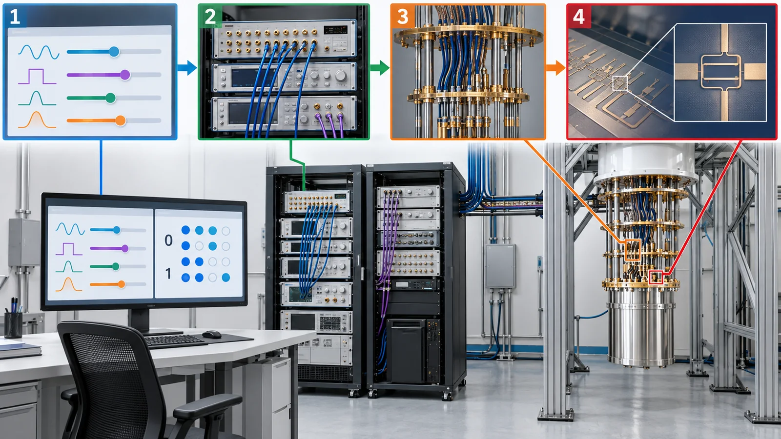
Kim et al. ran circuits of up to 60 layers of two-qubit gates (2,880 CNOT gates in total) on a 127-qubit superconducting processor (IBM Eagle) and measured expectation values using error mitigation (ZNE) Sourced[Ref. 18]. They first checked correctness on circuits that classical computers can verify exactly, then moved to circuits beyond brute-force classical simulation. The paper presents the result as evidence for the utility of quantum computing before fault tolerance Sourced[Ref. 18] (a company (IBM) claim).
Soon after the paper appeared, classical researchers showed efficient ways to compute the same problem. Tindall et al. reported a classical simulation, using a tensor network matched to the lattice, that is more accurate and precise than the quantum processor's results Sourced[Ref. 19]. Begušić et al. likewise reported that a method called sparse Pauli dynamics reproduces the results far faster than the reported quantum runtime, even on one laptop core Sourced[Ref. 20]. How to read this dispute (who claimed advantage, on which task, against what) is the subject of our explainer on reading claims of quantum advantage.
What it shows: with error mitigation, even a 127-qubit machine without error correction produced correct expectation values for particular circuits, to the extent that could be checked exactly (the paper's claim). What it does not show: that this calculation was faster than classical computing, in any settled sense, given the classical rebuttals. Nor is the circuit an industrial problem in itself (the paper says it does not aim at problems with proven speed-ups Sourced[Ref. 18]).
VQE was first tried on molecules (H₂, LiH, BeH₂) because the problem of electron energies maps directly onto qubit states Sourced[Ref. 5]. Targets that matter in materials work, such as the active sites of catalysts and magnetism, may involve strong electron correlation that is hard even for classical methods, which is where hopes lie (our commentary; see the explainer on quantum chemistry and materials simulation).
But materials engineers should check three things. (1) What it is compared with: classical methods such as density functional theory, or classical approximations of equal cost. (2) Scale: are the molecules tried small enough for classical computers to solve exactly (the examples in the table are small molecules)? (3) Measurement cost: the number of terms grows roughly as M⁴ and each takes thousands to millions of shots, so how much experiment time is needed (chapter 7)?
10. Limits, what we could not confirm, and a summary
(1) What we could not confirm
- The text of ISO/IEC 4879:2024 (quantum computing vocabulary) is paywalled, so we could not confirm whether it defines NISQ, variational algorithms or related terms. We confirmed only the number, title, publication month and scope statement on the ISO page.
- IEEE P3185 (hybrid quantum-classical computing), P7130 (definitions) and P7131 (performance metrics and benchmarking) appear on IEEE SA pages as projects in development; we could not confirm them as published standards.
- We could not find a third-party-verified case of VQE or QAOA showing a practical advantage.
- We do not cover company roadmaps (qubit counts, logical qubits, dates).
- NISQ means a mid-sized quantum computer that has errors and does not correct them. Judge it by whether errors are corrected, not by the qubit count Sourced
- Hybrid computing is a loop of short quantum circuits and classical tuning. VQE targets molecular energies and QAOA targets combinatorial optimization Sourced
- There are three walls: noise (even at a 0.1% error, 1,000 gates leave about a 37% success chance), barren plateaus, and measurement counts (ten times the precision needs a hundred times the shots) Our calculation
- Error mitigation is not error correction. It corrects averages, and its cost rises exponentially with depth Sourced
- The real experiment (IBM, 127 qubits) was reproduced from the classical side. Read advantage as "who, on which task, against what" Sourced
11. How to read evaluations and standards
The performance of NISQ and hybrid computing is measured with several yardsticks. The error rate (the size of the error per gate, measured by randomized benchmarking) measures the quality of components. Quantum volume folds the number of qubits, errors and connectivity into one number for the quality of the whole machine. Application-oriented benchmarks measure how well real algorithms run. Each measures something different and leaves something else unmeasured. Checked on 16 October 2026.
| Item | Representative benchmarks and methods (name, source) | Standards and guidance (ISO/IEC, IEEE, etc.) | Reading notes |
|---|---|---|---|
| Gate error | Randomized benchmarking (Knill et al. 2008; Magesan et al. 2011) [Refs. 24, 25]Sourced | Not found (we did not find an international standard fixing the method) | Check which gate (one- or two-qubit), average or best, and over how many |
| Whole-machine quality | Quantum volume (Cross et al. 2019) [Ref. 26]; re-examination of the test (Baldwin et al. 2022) [Ref. 27]Sourced | Not found | One number does not predict performance on every application |
| Speed | CLOPS (circuit layer operations per second) proposed by Wack et al. 2021 [Ref. 28]Sourced | Not found | Includes the classical-side time (compiling, data transfer) |
| Algorithm performance | Application-oriented benchmarks (Lubinski et al. 2023, open source) [Ref. 29]Sourced | IEEE P7131 (proposed standard for performance metrics and benchmarking; working group active) [Ref. 33]. ISO/IEC JTC 3/JSC 3A has a benchmarking working group (WG 2) [Ref. 31]SourcedNot yet confirmed | Results depend on which algorithms are chosen |
| Terminology | — (a terminology standard, not an evaluation) | ISO/IEC 4879:2024 "Information technology — Quantum computing — Vocabulary" (published May 2024) [Ref. 30]. IEEE P7130 (quantum technology definitions, in development) [Ref. 32]SourcedNot yet confirmed | The text is paywalled; we could not confirm whether it defines NISQ |
| Hybrid architecture | — | IEEE P3185 "Standard for Hybrid Quantum-Classical Computing" (a project defining the hardware and software architecture of hybrid environments; in development) [Ref. 32]Not yet confirmed | Not confirmed as published; requirements not checked |
| Checking mitigation results | Comparison with exactly verifiable circuits (Kim et al.) [Ref. 18]; classical reproduction (Tindall et al.; Begušić et al.) [Refs. 19, 20]; a community record (the quantum advantage tracker) [Ref. 34]Sourced | Not found | Separate company announcements from third-party checks |
| Progress in error correction | Logical error rate and its fall as the code distance grows, Λ (Google 2025: Λ = 2.14 ± 0.02) [Ref. 22]Sourced | → see the surface-code explainer | Check over how many rounds and shots, and compared with what |
The table's organisation is Our calculation (a summary). Numbers, titles and status were checked on the official ISO and IEEE SA pages (16 October 2026). Standards texts are paywalled, so we state only scope and no requirements.
Reading notes for materials engineers
- "How many qubits" alone does not tell you performance: read a NISQ device together with its error rate, circuit length and connectivity. Neither quantum volume nor application-oriented benchmarks summarise everything in one number [Refs. 26, 27, 29]
- Company announcements and third-party checks are different: IBM's 127-qubit experiment was a company claim, followed by reports of classical reproduction [Refs. 18, 19, 20]. The dispute can increasingly be followed in public records such as the quantum advantage tracker [Ref. 34].
- Standards are mostly in development or voluntary: many standards in this field (IEEE P3185, P7130, P7131 and others) are still being drafted, and even once published they generally bind only when cited in law or contracts (our commentary). Distinguish plans (in development) from achievements (published).
12. Glossary
- NISQ
- Noisy Intermediate-Scale Quantum: a mid-sized quantum computer that has errors and does not correct them.
- Noise
- Slips of the qubit arrow caused by the environment or imperfect operations.
- Decoherence
- The gradual loss of the quantum state through the environment (the arrow wobbles).
- Fidelity
- How close an operation or state is to the ideal. One minus fidelity is the error.
- Gate
- An operation that rotates the qubit arrow.
- Measurement (shot)
- Looking at the arrow and settling on 0 or 1. One run is a shot.
- Expectation value
- The average of the outcomes of many shots.
- Hybrid computing
- Computation in which quantum and classical computers share the work.
- Variational quantum algorithm (VQA)
- Methods in which a classical computer tunes circuit knobs to lower a cost.
- VQE
- Variational Quantum Eigensolver: a VQA that searches for a system's lowest energy.
- QAOA
- Quantum Approximate Optimization Algorithm: a VQA for combinatorial optimization.
- Variational principle
- The principle that any state gives an average energy at or above the lowest energy.
- Hamiltonian
- The expression for a system's energy; on a quantum computer it is written as a sum of Pauli terms.
- Max-Cut
- Colour points in two colours to maximise the links joining different colours.
- Barren plateau
- A landscape that is nearly flat, with gradients that shrink exponentially.
- Gradient
- The rate at which the cost changes when a knob is nudged (the slope).
- Error suppression
- Methods that make errors less likely during the run (dynamical decoupling, etc.).
- Error mitigation
- Methods that correct the averaged results after the run (ZNE, PEC, etc.).
- ZNE
- Zero-noise extrapolation: measure with more noise and extrapolate to zero noise.
- PEC
- Probabilistic error cancellation: mix in inverse-noise operations at random.
- Dynamical decoupling
- Short pulses applied while a qubit waits to cancel environmental fluctuations.
- Error correction
- Protecting one logical qubit with many physical qubits and fixing errors during the run.
- Quantum volume
- A single number for whole-machine quality that combines qubits, errors and connectivity.
13. References
- Preskill J. "Quantum Computing in the NISQ era and beyond", Quantum 2, 79 (2018), DOI 10.22331/q-2018-08-06-79 — doi.org/10.22331/q-2018-08-06-79
- Bharti K. et al. "Noisy intermediate-scale quantum (NISQ) algorithms", Rev. Mod. Phys. 94, 015004 (2022), DOI 10.1103/RevModPhys.94.015004 — doi.org/10.1103/RevModPhys.94.015004
- Cerezo M. et al. "Variational quantum algorithms", Nat. Rev. Phys. 3, 625–644 (2021), DOI 10.1038/s42254-021-00348-9 — doi.org/10.1038/s42254-021-00348-9
- Peruzzo A. et al. "A variational eigenvalue solver on a quantum processor", Nat. Commun. 5, 4213 (2014), DOI 10.1038/ncomms5213 (open access) — doi.org/10.1038/ncomms5213
- Kandala A. et al. "Hardware-efficient variational quantum eigensolver for small molecules and quantum magnets", Nature 549, 242–246 (2017), DOI 10.1038/nature23879 — doi.org/10.1038/nature23879
- Farhi E., Goldstone J., Gutmann S. "A Quantum Approximate Optimization Algorithm", arXiv:1411.4028 (2014) — arxiv.org/abs/1411.4028
- McArdle S. et al. "Quantum computational chemistry", Rev. Mod. Phys. 92, 015003 (2020), DOI 10.1103/RevModPhys.92.015003 — doi.org/10.1103/RevModPhys.92.015003
- McClean J. R. et al. "Barren plateaus in quantum neural network training landscapes", Nat. Commun. 9, 4812 (2018), DOI 10.1038/s41467-018-07090-4 (open access) — doi.org/10.1038/s41467-018-07090-4
- Cerezo M. et al. "Cost function dependent barren plateaus in shallow parametrized quantum circuits", Nat. Commun. 12, 1791 (2021), DOI 10.1038/s41467-021-21728-w (open access) — doi.org/10.1038/s41467-021-21728-w
- Wang S. et al. "Noise-induced barren plateaus in variational quantum algorithms", Nat. Commun. 12, 6961 (2021), DOI 10.1038/s41467-021-27045-6 (open access) — doi.org/10.1038/s41467-021-27045-6
- Cerezo M. et al. "Does provable absence of barren plateaus imply classical simulability?", Nat. Commun. 16, 7907 (2025), DOI 10.1038/s41467-025-63099-6 — doi.org/10.1038/s41467-025-63099-6
- Stilck França D., García-Patrón R. "Limitations of optimization algorithms on noisy quantum devices", Nat. Phys. 17, 1221–1227 (2021), DOI 10.1038/s41567-021-01356-3 — doi.org/10.1038/s41567-021-01356-3
- Temme K., Bravyi S., Gambetta J. M. "Error mitigation for short-depth quantum circuits", Phys. Rev. Lett. 119, 180509 (2017), DOI 10.1103/PhysRevLett.119.180509 — doi.org/10.1103/PhysRevLett.119.180509
- Cai Z. et al. "Quantum error mitigation", Rev. Mod. Phys. 95, 045005 (2023), DOI 10.1103/RevModPhys.95.045005 — doi.org/10.1103/RevModPhys.95.045005
- Takagi R., Endo S., Minagawa S., Gu M. "Fundamental limits of quantum error mitigation", npj Quantum Inf. 8, 114 (2022), DOI 10.1038/s41534-022-00618-z (open access) — doi.org/10.1038/s41534-022-00618-z
- Quek Y. et al. "Exponentially tighter bounds on limitations of quantum error mitigation", Nat. Phys. 20, 1648–1658 (2024), DOI 10.1038/s41567-024-02536-7 — doi.org/10.1038/s41567-024-02536-7
- Ezzell N. et al. "Dynamical decoupling for superconducting qubits: a performance survey", Phys. Rev. Applied 20, 064027 (2023), DOI 10.1103/PhysRevApplied.20.064027 — doi.org/10.1103/PhysRevApplied.20.064027
- Kim Y. et al. "Evidence for the utility of quantum computing before fault tolerance", Nature 618, 500–505 (2023), DOI 10.1038/s41586-023-06096-3 — doi.org/10.1038/s41586-023-06096-3
- Tindall J., Fishman M., Stoudenmire E. M., Sels D. "Efficient tensor network simulation of IBM's Eagle kicked Ising experiment", PRX Quantum 5, 010308 (2024), DOI 10.1103/PRXQuantum.5.010308 — doi.org/10.1103/PRXQuantum.5.010308
- Begušić T., Gray J., Chan G. K.-L. "Fast and converged classical simulations of evidence for the utility of quantum computing before fault tolerance", Sci. Adv. 10, eadk4321 (2024), DOI 10.1126/sciadv.adk4321 — doi.org/10.1126/sciadv.adk4321
- Arute F. et al. "Quantum supremacy using a programmable superconducting processor", Nature 574, 505–510 (2019), DOI 10.1038/s41586-019-1666-5 (open access) — nature.com/articles/s41586-019-1666-5
- Google Quantum AI "Quantum error correction below the surface code threshold", Nature 638, 920–926 (2025), DOI 10.1038/s41586-024-08449-y — nature.com/articles/s41586-024-08449-y
- Gao D. et al. "Establishing a new benchmark in quantum computational advantage with 105-qubit Zuchongzhi 3.0 processor", Phys. Rev. Lett. 134, 090601 (2025), arXiv:2412.11924 — arxiv.org/abs/2412.11924
- Knill E. et al. "Randomized benchmarking of quantum gates", Phys. Rev. A 77, 012307 (2008), DOI 10.1103/PhysRevA.77.012307 — doi.org/10.1103/PhysRevA.77.012307
- Magesan E., Gambetta J. M., Emerson J. "Scalable and robust randomized benchmarking of quantum processes", Phys. Rev. Lett. 106, 180504 (2011), DOI 10.1103/PhysRevLett.106.180504 — doi.org/10.1103/PhysRevLett.106.180504
- Cross A. W. et al. "Validating quantum computers using randomized model circuits", Phys. Rev. A 100, 032328 (2019), DOI 10.1103/PhysRevA.100.032328 — doi.org/10.1103/PhysRevA.100.032328
- Baldwin C. H. et al. "Re-examining the quantum volume test: Ideal distributions, compiler optimizations, confidence intervals, and scalable resource estimations", Quantum 6, 707 (2022), DOI 10.22331/q-2022-05-09-707 — doi.org/10.22331/q-2022-05-09-707
- Wack A. et al. "Quality, Speed, and Scale: three key attributes to measure the performance of near-term quantum computers", arXiv:2110.14108 (2021) — arxiv.org/abs/2110.14108
- Lubinski T. et al. "Application-oriented performance benchmarks for quantum computing", IEEE Trans. Quantum Eng. 4, 1–32 (2023), DOI 10.1109/TQE.2023.3253761 — doi.org/10.1109/TQE.2023.3253761
- ISO/IEC "ISO/IEC 4879:2024 Information technology — Quantum computing — Vocabulary" (ISO catalogue page) — iso.org/standard/80432.html
- IEC/ISO JTC 3/JSC 3A "Quantum computing" (committee page: scope and working groups WG 1 supply chain, WG 2 benchmarking, WG 3 terminology and quantities) — iso.org/committee/12010875.html
- IEEE SA "IEEE Standards & Projects for Quantum Technologies" (lists P3185 Hybrid Quantum-Classical Computing, P7130 Quantum Technologies Definitions, P3329 energy efficiency) — standards.ieee.org/initiatives/quantum-standards-activities/
- IEEE SA "Quantum Benchmarking Working Group P7131" (working group site; technical scope defined by P7131) — sagroups.ieee.org/7131/
- Gambetta J., Davis R. (IBM) "Quantum advantage tracker" (IBM Quantum blog, 23 February 2026) — ibm.com/quantum/blog/quantum-advantage-tracker
14. Claim-to-source audit
| Claim in the text | Basis | Category |
|---|---|---|
| Preskill proposed the term NISQ in 2018 and said that machines of 50-100 qubits may surpass classical computers on some tasks while gate noise limits circuit size | Reference 1 https://doi.org/10.22331/q-2018-08-06-79 | Sourced |
| The review description of NISQ computers as made of hundreds of noisy qubits, not error-corrected, operating only within a limited coherence time | Reference 2 https://doi.org/10.1103/RevModPhys.94.015004 | Sourced |
| The definition of variational quantum algorithms (a classical optimizer trains a parametrized circuit) and their challenges of trainability, accuracy and efficiency | Reference 3 https://doi.org/10.1038/s42254-021-00348-9 | Sourced |
| The photonic-processor experiment in which VQE gave the HeH⁺ ground-state energy to chemical accuracy (Peruzzo et al. 2014) | Reference 4 https://doi.org/10.1038/ncomms5213 | Sourced |
| Up to six qubits and over a hundred Pauli terms, with H₂, LiH, BeH₂ ground-state energies and a magnetism problem; agreement with noisy-device simulation | Reference 5 https://doi.org/10.1038/nature23879 | Sourced |
| The proposal of QAOA; p-layer circuits; a cut at least 0.6924 times the optimum for p = 1 on 3-regular graphs | Reference 6 https://arxiv.org/abs/1411.4028 | Sourced |
| The number of Pauli terms grows roughly as the fourth power of orbitals in a Gaussian basis; chemical accuracy is 1.6×10⁻³ hartree | Reference 7 https://doi.org/10.1103/RevModPhys.92.015003 | Sourced |
| For a wide class of circuits the probability of a non-zero gradient shrinks exponentially with qubit count (barren plateaus) | Reference 8 https://doi.org/10.1038/s41467-018-07090-4 | Sourced |
| Global cost functions give barren plateaus even in shallow circuits; local cost functions give polynomially vanishing gradients up to depth O(log n) | Reference 9 https://doi.org/10.1038/s41467-021-21728-w | Sourced |
| Under local Pauli noise, with depth growing linearly in n, the gradient vanishes exponentially (noise-induced barren plateaus) | Reference 10 https://doi.org/10.1038/s41467-021-27045-6 | Sourced |
| The argument that circuits structured to avoid barren plateaus can often be simulated efficiently by classical computers | Reference 11 https://doi.org/10.1038/s41467-025-63099-6 | Sourced |
| On noisy devices, substantial quantum advantage in classical optimization is unlikely unless noise falls by orders of magnitude or the topology matches | Reference 12 https://doi.org/10.1038/s41567-021-01356-3 | Sourced |
| The proposal of ZNE and a second noise-cancelling method (PEC) for short-depth circuits | Reference 13 https://doi.org/10.1103/PhysRevLett.119.180509 | Sourced |
| The review of error mitigation: methods that soften rather than fully remove errors in the NISQ era | Reference 14 https://doi.org/10.1103/RevModPhys.95.045005 | Sourced |
| For layered circuits with local depolarizing noise the sample overhead grows exponentially with depth (Takagi et al.); a superpolynomial number of samples is needed in the worst case even for shallow circuits (Quek et al.) | Reference 15 https://doi.org/10.1038/s41534-022-00618-z Reference 16 https://doi.org/10.1038/s41567-024-02536-7 | Sourced |
| Dynamical decoupling as the simplest and least resource-intensive error suppression; 60 sequences compared on three IBM devices | Reference 17 https://doi.org/10.1103/PhysRevApplied.20.064027 | Sourced |
| The 127-qubit, up-to-60-layer, 2,880-CNOT experiment; the use of ZNE with probabilistic error amplification; why PEC was not used; TLS-driven drift; median T₁ = 288 µs and T₂ = 127 µs; the paper's framing as evidence of utility (a company claim) | Reference 18 https://doi.org/10.1038/s41586-023-06096-3 | Sourced |
| Classical reproductions: tensor networks (Tindall et al.) and sparse Pauli dynamics (Begušić et al.) | Reference 19 https://doi.org/10.1103/PRXQuantum.5.010308 Reference 20 https://doi.org/10.1126/sciadv.adk4321 | Sourced |
| The stated two-qubit gate fidelity of 99.62% for Zuchongzhi 3.0 | Reference 23 https://arxiv.org/abs/2412.11924 | Sourced |
| The predicted fidelity of 0.2% for the 53-qubit circuits, and the XEB uncertainty of 1/√(number of samples) | Reference 21 https://www.nature.com/articles/s41586-019-1666-5 | Sourced |
| Λ = 2.14 ± 0.02 reduction of the logical error rate per +2 in code distance; 0.143% error per cycle for the 101-qubit distance-7 code | Reference 22 https://www.nature.com/articles/s41586-024-08449-y | Sourced |
| The proposals of randomized benchmarking, quantum volume, CLOPS and application-oriented benchmarks, and the re-examination of the quantum volume test | Reference 24 https://doi.org/10.1103/PhysRevA.77.012307 Reference 25 https://doi.org/10.1103/PhysRevLett.106.180504 Reference 26 https://doi.org/10.1103/PhysRevA.100.032328 Reference 27 https://doi.org/10.22331/q-2022-05-09-707 Reference 28 https://arxiv.org/abs/2110.14108 Reference 29 https://doi.org/10.1109/TQE.2023.3253761 | Sourced |
| ISO/IEC 4879:2024 (quantum computing vocabulary): number, title, May 2024 publication and scope | Reference 30 https://www.iso.org/standard/80432.html | Sourced |
| The scope of ISO/IEC JTC 3/JSC 3A (including annealers and hybrid forms) and its working groups on supply chain, benchmarking and terminology | Reference 31 https://www.iso.org/committee/12010875.html | Sourced |
| IEEE P3185 (hybrid quantum-classical computing), P7130 (definitions) and P3329 (energy efficiency) are listed as IEEE SA quantum projects; the technical scope of the P7131 working group | Reference 32 https://standards.ieee.org/initiatives/quantum-standards-activities/ Reference 33 https://sagroups.ieee.org/7131/ | Sourced |
| The quantum advantage tracker (IBM blog, February 2026) as a public record of candidates | Reference 34 https://www.ibm.com/quantum/blog/quantum-advantage-tracker | Sourced |
| The (1−ε)^N table and Fig. 2 (0.1% and 1,000 gates → about 37%; 1% → about 0.004%; N for 50% about 69, 693, 6,931; 99.62% → about 182) | Our calculation (a simple model assuming independent errors) | Our calculation |
| The one-qubit VQE example (E(θ) = cos θ, standard error 0.10 for 100 shots), the shot-count table (M = (σ ÷ precision)²), the made-up ZNE example (0.967, 1.000, √5 ≈ 2.24), the Max-Cut example (5 points, 6 links, maximum 5, 32 colourings, 4 optima) and the 2⁻ⁿ illustration | Our calculation (Python brute force and arithmetic; made-up values for illustration, not device results) | Our calculation |
| Whether ISO/IEC 4879 defines NISQ and related terms, whether IEEE P3185, P7130 and P7131 are published, third-party-verified practical advantage of VQE or QAOA, and company roadmaps | Not confirmed in the primary sources reachable for this article, so not stated | Commentary |
| The readings: the radio-knob analogy, the caveat on the variational principle, "mitigation is not correction", "reducing materials defects is the surest way to cut mitigation cost", and the division of roles | This article's commentary based on published material; not views stated by the institutions | Commentary |
| Fig. 2, Fig. 5, Fig. 6 and Fig. 9 are illustrations rather than real data; Fig. 3, Fig. 4, Fig. 7 and Fig. 8 are concept diagrams; Fig. 1 and Fig. 10 are ImageGen-generated conceptual illustrations | A note in this article | Commentary |
Last updated: 16 October 2026. Sources are limited to primary material (peer-reviewed papers, arXiv papers, official ISO and IEEE pages, official company blogs). Numerical examples are our own calculations, not device results. We could not confirm the text of ISO/IEC 4879, the publication status of IEEE P3185, P7130 and P7131, third-party-verified practical advantage of VQE or QAOA, or company roadmaps, so we do not state them. All figures are illustrative concept diagrams or drawings that include our calculations; Fig. 1 and Fig. 10 are ImageGen-generated conceptual illustrations.