TROY TECHNICAL · START HERE
(Read This First)
A Big-Picture Guide to Quantum Computing
What is different? Why the excitement? What is still difficult?
Understand the landscape before learning the equations.
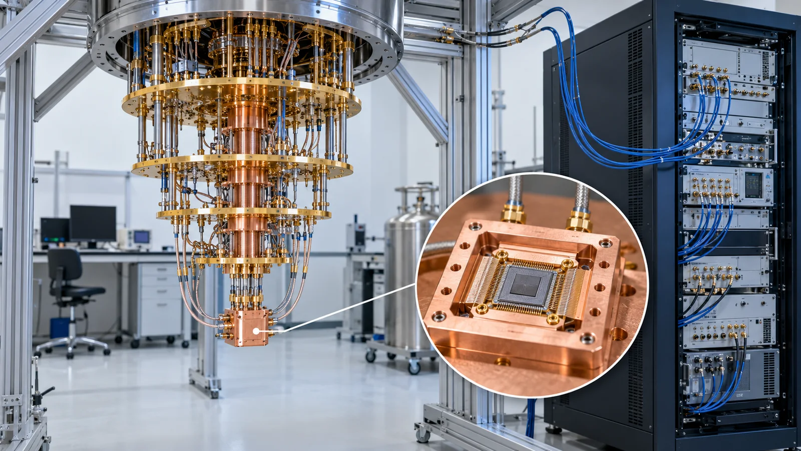
You may have heard that quantum computers could outperform supercomputers. But faster at what? And why do the pictures feature refrigerators and lasers instead of familiar computer boxes?
Start here: a quantum computer is not an upgraded replacement for every conventional computer. It handles information differently, making different methods possible for particular kinds of calculation. This guide connects the promise and the limitations. The individual articles linked at the end cover the machinery and mathematics in depth.
01 What changes from conventional computing?
Phones, laptops and supercomputers handle information as bits. A bit has the value 0 or 1; sequences of bits can represent text or pictures. In this comparison, these machines are called classical computers. “Classical” does not mean obsolete: it includes today’s CPUs and GPUs.
Quantum computers use quantum bits, or qubits. Information is encoded in quantum states of atoms, light, tiny electrical circuits or other physical systems. Quantum mechanics also underlies ordinary semiconductors; the distinctive step in quantum computing is to preserve and use features such as superposition and interference as computational resources.[1]
Classical machines already process many things in parallel and exploit sophisticated problem-specific shortcuts. A quantum advantage must be assessed against classical methods that include those capabilities.
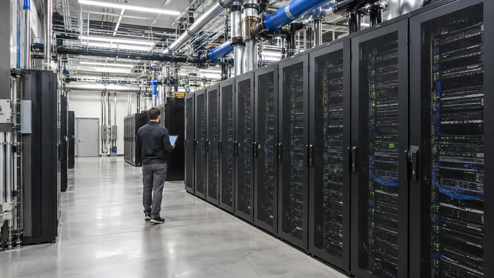
| Question | Classical computing | Quantum computing |
|---|---|---|
| What is manipulated? | Bit values, using logic and other operations. Parallelism and randomness are available too. | Quantum states, using interference of amplitudes and other quantum features. |
| What can be read? | Recorded bit strings. | Ordinary 0/1 measurements yield bit strings—not a complete list of amplitudes in one reading. |
| What role makes sense? | Everyday information processing, data management and a wide range of numerical work. | Potentially, selected tasks with a suitable quantum algorithm. |
This compares information-processing principles. It is not a performance benchmark showing that quantum hardware is superior.
02 What does using one look like?
The quantum device does not take over everything from entering a question to writing a report. Conventional computers remain at the entrance and exit. The device that performs the quantum part is called a QPU: quantum processing unit.
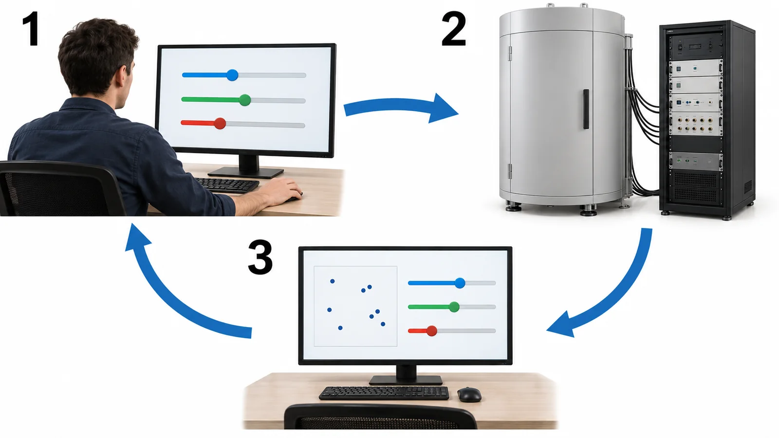
- Translate the question. A classical computer helps specify the desired result, prepare the quantum-state instructions and design a sequence of operations.
- Prepare, operate and measure. Electrical signals, lasers or other controls manipulate the qubits. Repeat the preparation-through-measurement sequence to gather the required statistics.
- Turn measurements into an answer. Classical processing estimates a quantity such as an energy. Some workflows update settings and repeat the process.[5]
The basic operations are quantum gates. A quantum circuit depicts their sequence using lines and symbols. It represents instructions, not a photograph of physical wiring.[8]
A useful starting picture is a classical computer working with a device that has different computational strengths. This does not mean that an existing GPU program can simply be sent to a QPU.
03 Three ideas behind the mechanism
This is the conceptual hurdle. Focus on what each feature does in a calculation, rather than memorizing equations.
Superposition: not just an unread 0 or 1
A qubit can be in state 0, state 1 or a superposition of them. It is not a bag containing two completed answers that you can both retrieve. The state is described using quantities called amplitudes, from which measurement probabilities are obtained.[2]
Unlike ordinary probabilities, amplitudes can reinforce or cancel one another, like waves. Their relative alignment is described by phase. Two states with the same 0/1 measurement probabilities need not be the same quantum state.
Interference: turn wave-like addition into a method
Think of ripples: a crest meeting a crest reinforces the disturbance; a crest meeting a trough can weaken it. Quantum computation uses interference of amplitudes to make a desired property accessible through measurement. Actual water waves are not being poured through a chip.
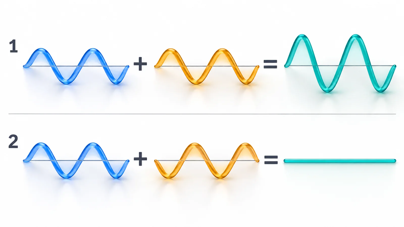
Crucially, the machine does not already know which answer is correct and magically choose it. People must use the structure of the problem to design a sequence of operations: a quantum algorithm. Preparing superposition without a useful method is not enough.[3]
A small check: how is this different from a fifty-fifty lottery?
Start a qubit in 0 and apply an operation called H, or Hadamard. Each case ends with a 0/1 measurement.
- One H:0 and 1 each have a 50% probability.
- Two H operations, with no measurement between: interference produces 0 with 100% probability and 1 with 0%.
- H → 0/1 measurement → H: the final probabilities are 50% each again. The intermediate measurement changes the state needed for the subsequent interference.
A lottery whose behavior is unchanged by checking it midway does not capture this distinction. These are calculated ideal values for standard quantum operations, not hardware measurements. This tiny example does not itself demonstrate a computational speedup.[2]
Entanglement: describe the whole, not separate parts
Qubits can be entangled: their joint state cannot be described as separate, independent states. In one two-qubit example, a 0/1 measurement gives either 00 or 11 with equal probability. Matching outcomes alone are not proof of entanglement; classical systems can do that too. The distinction involves correlations across different choices of measurement.[4]
For now, remember: the collection is manipulated as a joint state, including relationships between its parts. Entanglement does not let someone send a chosen message faster than light.[14]
04 Why can’t we read every answer?
Three qubits have eight possible 0/1 strings, from 000 to 111. Amplitudes for those strings describe the joint state. But an ordinary measurement of all three gives one three-bit string per run, not a printout of eight amplitudes or eight answers.[4]
Repeatedly prepare the same state, perform the same operations and measure: patterns in the outcomes become apparent. Those repetitions take time too. Measurement generally changes the state, so intermediate quantum data cannot be freely inspected.[2]
It is to obtain useful information through limited readout.
The result need not be one “correct candidate.” A calculation might estimate a molecular energy or sample a distribution with a particular property.
This is why a quantum computer is neither unlimited readable memory nor an instant brute-force search engine.[12]
05 Where could it help—and where not?
“Hard for a classical computer” does not automatically mean “good for quantum computing.” A suitable method, the required accuracy and a favorable end-to-end cost all matter.
The prospective advantage is not simply executing the same instructions at a higher clock rate. For some problems, quantum algorithms greatly reduce how the required work grows as the input gets larger. That is a different kind of opportunity—but not a shortcut available for every problem.[6][7]
A tangible example: understanding molecules and materials
Suppose you are investigating a catalyst. You need more than a picture of a molecule: you want electronic properties or energies relevant to a reaction. Electrons behave quantum mechanically, and faithfully calculating their interactions can become difficult for classical machines.
Use a controllable quantum system to calculate the behavior of another quantum system: that is the motivation for quantum simulation. It is not a finished-product generator. Researchers still need a model, a way to extract the desired quantities, and checks against classical calculations and experiments. A speedup is not guaranteed for every chemistry problem.[3]
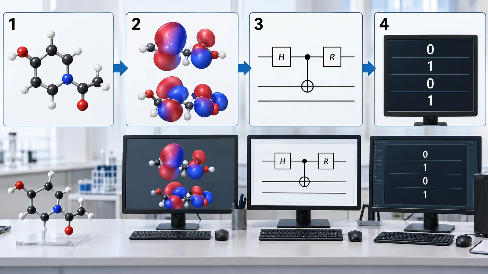
AN IMPORTANT THEORETICAL EXAMPLE
Particular mathematical problems
With sufficiently large and reliable hardware, Shor’s algorithm efficiently factors large integers and solves certain related problems. This is a major reason to expect advantages over known classical methods—not evidence that today’s machines can immediately break practical cryptography.[6]
CHECK THE CONDITIONS
Search, optimization and AI
Grover’s search reduces the theoretical number of calls to an operation that tests a condition. Constructing that operation and preparing data still matter. The labels “optimization” and “AI” alone do not establish a faster real-world workflow.[7][15]
A useful starting list of poor targets: email, spreadsheets, storing pictures and browsing the web—work classical computers already perform efficiently. The question is which particular part of a workload would benefit.
06 Why is it so difficult?
Environmental disturbances and imperfect control can change quantum states. If phase relationships or other intended properties are lost, the required interference and correlations are no longer reliable. The information needs isolation, yet computation requires precise interaction and measurement. Reconciling those demands is difficult.[9][10]
More qubits are not enough
A physical qubit is an actual component, such as a circuit or an atom. A logical qubit is a unit of quantum information encoded across multiple physical qubits and protected against errors.
Error correction repeatedly collects and processes checks that reveal errors without directly reading the protected information. It does not perfectly copy an unknown quantum state and vote among the copies. Extra qubits, checks and classical processing are needed. Their overhead depends on the code, error rates and length of the calculation.[8][10]
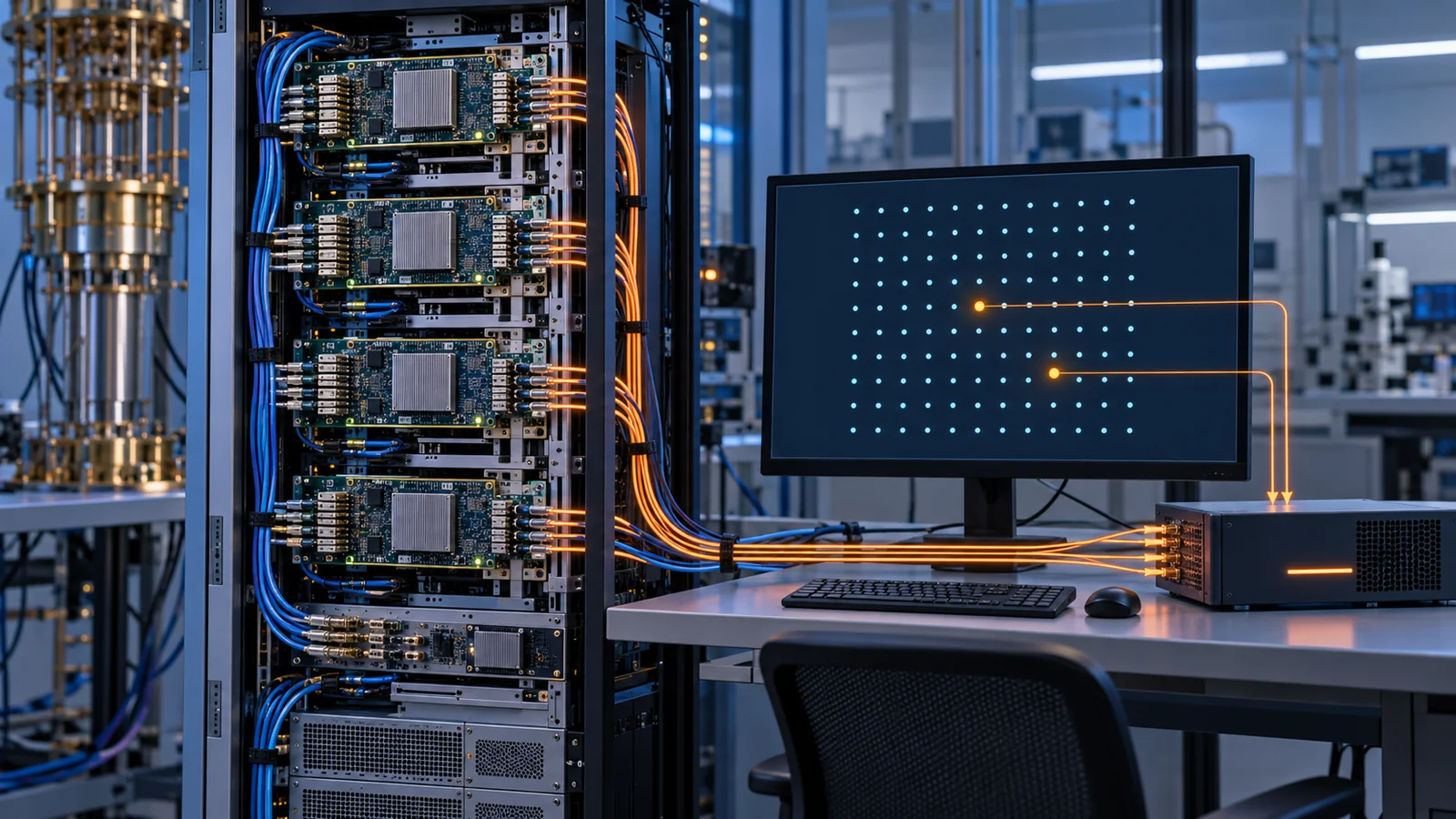
Coherence concerns preservation of quantum relationships needed for computation; fidelity quantifies closeness to an intended state or operation. Quality and the amount of reliable computation matter alongside qubit count.[9]
Fewer theoretical steps may not mean an earlier answer
Input preparation, translation into hardware operations, repeated measurements, handling errors and post-processing all consume resources. A favorable quantum subroutine can still leave an unfavorable overall time or cost.[5]
For the same problem at the same accuracy, how do total time, cost and resources—from preparation to answer—compare with well-optimized classical methods? This guide proposes that as a useful decision framework.
07 Does every quantum computer need that refrigerator?
No. The familiar hanging assembly of gold-colored wiring belongs to cooling equipment used by superconducting systems and some other approaches. The choice of physical qubit changes the surrounding machinery. There is no single appearance shared by all quantum computers.[12]
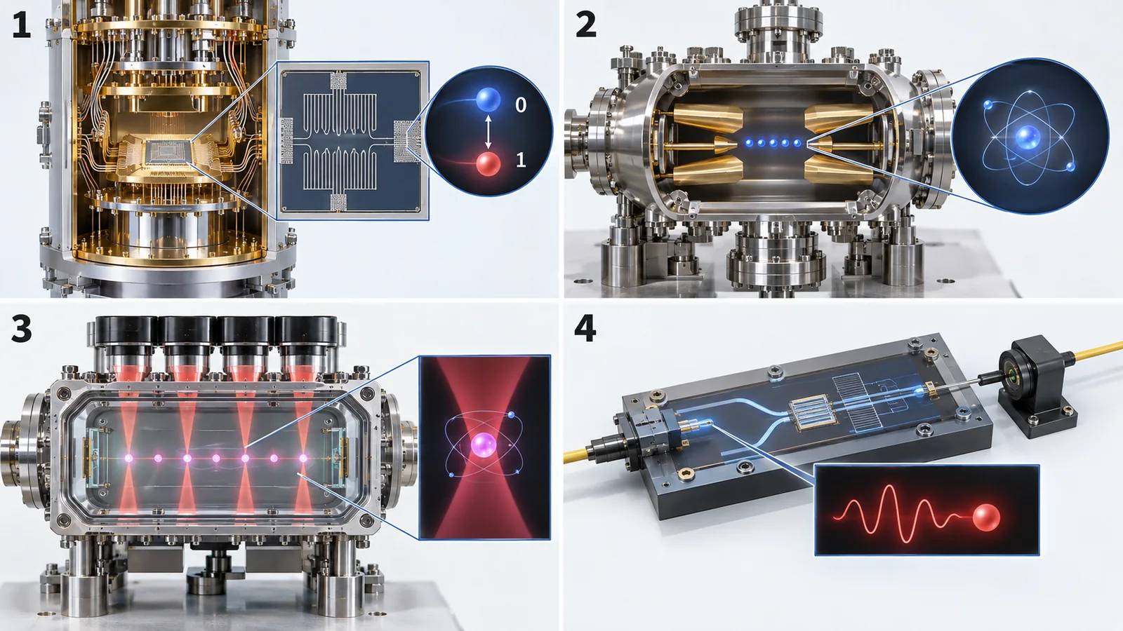
Circuits and semiconductors
Approaches include superconducting circuits and electrons confined in silicon. Fabrication, interfaces, wiring and low-temperature control matter.
Atoms and light
Other approaches hold and manipulate ions or neutral atoms, or encode information in photons. They involve combinations of vacuum systems, lasers, optical circuits and detectors.[12]
These are not simply identical qubits arranged by competing companies. Gate speed, errors, connectivity and manufacturability involve different trade-offs. Rather than choosing a winner immediately, see the supporting apparatus and materials as part of the computing system.
08 How should we read the current state of the field?
Neither “nothing exists” nor “everything is ready” is a useful description. Real hardware can run circuits through cloud services, and error-correction experiments are progressing. For example, Google Quantum AI and collaborators reported lower logical error rates as particular surface-code memories were enlarged. That is an important advance, not by itself a demonstration of long general-purpose computations or broad industrial advantage.[5][11]
NISQ means noisy intermediate-scale quantum technology: errors still limit computation. Fault-tolerant quantum computing aims to use error correction during operations to maintain sufficiently low logical error rates. There is no single qubit-count boundary separating the two for every machine.[9][10]
Also separate a quantum-advantage demonstration on a narrow task from a benefit in a working business process. Better classical algorithms can change comparisons. Rather than naming one universal arrival date, ask which problem was tested, and under which conditions.[12]
Four questions for an impressive headline
- What is counted? Physical qubits or logical qubits?
- What was demonstrated? Memory, short operations, a long computation or a useful application?
- Compared with what? Which classical method, accuracy, input size and definition of elapsed time?
- Result or plan? Distinguish experiments, conditional estimates and company targets.
This is this guide’s suggested reading framework, not a ranking of machines.
09 Similar names, different purposes
This guide mainly discusses gate-based quantum computing, in which operations are combined in sequence. Related technologies serve different purposes.
- Quantum annealing
- Encodes a problem in the search for low-energy states. It differs from the gate-model story above; practical benefits depend on the problem and comparison. → Quantum annealing
- Quantum communication and networks
- Use quantum states or correlations across locations. They do not make communication faster than light. → Quantum networks and repeaters
- Quantum sensing
- Uses sensitivity to the environment to measure quantities such as magnetic fields. Its purpose differs from speeding up computation. → Quantum sensing
These are brief signposts within the series. Follow the individual articles for their mechanisms and sources.
10 Follow your next question
You do not need to read all 36 articles in order. Try big picture → your question → the components you need. Choose one of these short routes.
Understand the mechanism
Follow the concepts through small diagrams and numerical examples.
Could it help in practice?
Start with applications, then learn to assess advantage claims.
What makes reliable operation hard?
Go from state quality to error correction and logical qubits.
Explore devices and materials
Start with materials and fabrication, then choose a hardware approach.
Try the workflow
Understand classical–quantum coordination before exploring cloud access.
Understand the security implications
Begin with PQC and migration, then distinguish quantum communication.
Open the complete map of 36 technical explainers
These groups are editorial navigation for this overview. Supporting materials and fabrication articles cover enabling technologies; they are not all articles about qubits themselves.
Principles and workflow
- Quantum computing fundamentals: diagrams and small examples
- Quantum gates and circuits
- Quantum algorithms
- Coherence and fidelity
- NISQ and hybrid computing
- Software and cloud access
Reliability and error correction
Physical qubit approaches
- Superconducting qubits
- Trapped ions
- Neutral atoms
- Silicon spin qubits
- Photonic quantum computing
- Topological quantum computing
Applications and evaluation
- Quantum chemistry and materials simulation
- Industrial applications: what is realistic?
- How to read quantum-advantage claims
- Quantum annealing
Security, networks and sensing
- Post-quantum cryptography
- Migrating to post-quantum cryptography
- Quantum key distribution and communication
- Quantum networks and repeaters
- Quantum sensing
Materials, fabrication and optics
- Materials and fabrication for quantum computers
- Quantum dots
- Atomic layer deposition
- Nanoscale metrology
- Spintronic materials
- Thin-film lithium niobate
- Silicon nitride waveguides
- Silicon photonics
- Photodetectors
- Semiconductor lasers
- Optical fiber
Strategy and policy
11 The picture to take away
A quantum computer controls quantum states to solve selected computational tasks differently. Superposition alone is not enough: interference, entanglement and an appropriate method help extract useful information from limited measurements.
That creates real possibilities where the method fits. It also brings difficult errors, readout overhead and competition from classical computing. Think “a different computational technology whose useful role must be identified,” not “a magic faster laptop.” The individual articles on devices, algorithms and materials then become parts of the same landscape.
Sources and scope
Codex wrote this overview from scratch as an entry point to the existing series. Educational sources and original papers support the principles; the cited experimental paper supports the specific research example. Analogies, comparisons, reading routes and headline questions are this guide’s explanatory and editorial synthesis. This is not an exhaustive news survey after the check date, nor a blanket judgment on practical advantage for every device.
Six illustrations reuse existing ImageGen assets; one new wave-addition illustration was generated for this guide to explain interference. They are not photographs of actual hardware, measurements or construction drawings of real products. Read the numbered elements and enlarged models together with their captions. Both language editions use identical image files, with no additional generation for the English edition.
Primary and educational sources, with reading purpose
- IBM Quantum Learning. Quantum computing fundamentalsBits, qubits and the introductory principles.
- IBM Quantum Learning. Quantum information — single systemsAmplitudes, measurement, phase and H. Ideal example values calculated for this guide.
- Ashley Montanaro (2016). Quantum algorithms: an overviewAlgorithm families, applications and conditional speedups.
- IBM Quantum Learning. Quantum information — multiple systemsJoint states, entanglement and measured bit strings.
- IBM Quantum Learning. Running quantum circuitsClassical–quantum workflow, mapping, execution and post-processing.
- Peter W. Shor (1997). Polynomial-Time Algorithms for Prime Factorization and Discrete Logarithms on a Quantum ComputerEfficient quantum algorithms for factoring and discrete logarithms.
- Lov K. Grover (1996). A fast quantum mechanical algorithm for database searchSearch query complexity, distinguished here from end-to-end runtime.
- IBM Quantum Learning. Quantum circuitsQuantum circuits and the no-cloning theorem for arbitrary unknown states.
- John Preskill (2018). Quantum Computing in the NISQ era and beyondMeaning of NISQ and limitations from noise; not used for current device counts.
- IBM Quantum Learning. Correcting quantum errors — introduction; Noise and errorsFragility and error correction. Also see Noise and errors and Error correction I.
- R. Acharya et al., Google Quantum AI and collaborators (2024). Quantum error correction below the surface code thresholdAn experimental example of decreasing logical error with larger surface-code memories.
- NIST (updated 28 May 2026). Quantum Computing ExplainedReadout limitations, hardware approaches and research versus practical use.
- NIST (13 August 2024). NIST Releases First 3 Finalized Post-Quantum Encryption StandardsFinalization of three PQC standards, distinguished from using quantum hardware.
- IBM Quantum Learning. Quantum TeleportationWhy entanglement does not enable faster-than-light messaging.
- IBM Quantum Learning. Quantum machine learning — introductionWhy tasks already handled well classically are not automatic quantum-speedup targets.