TECHNOLOGY EXPLAINER
Software and Cloud Access
— The tools for "using" a quantum computer, and how access works
Quantum computers sit in distant laboratories or in refrigerators inside data centres. So how do the rest of us use one? The answer: write a "circuit" on your own computer, send it over the network (the cloud), and receive the result. This article explains, with figures and small examples we actually ran: (1) what a quantum program is (what it means to "write a circuit"), (2) a map of software development kits (SDKs) such as Qiskit, Cirq and CUDA-Q, (3) the compiler (transpiler) that rewrites an ideal circuit for a real machine, (4) how cloud use works and what "shots" means, and (5) hybrid execution that combines quantum and classical computers. We do not rank products. For materials engineers we add the link to materials computation and a few cautions on handling data.
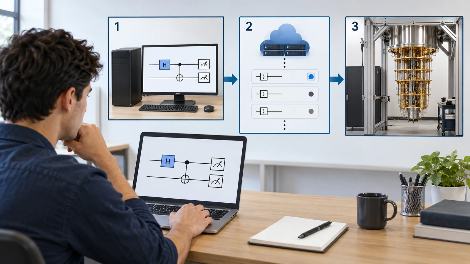
- The short version, what to know first, and where this fits in the series
- What a quantum program is — "writing a circuit"
- A map of SDKs — Qiskit, Cirq, CUDA-Q and others
- Compilers and transpilers — turning the "ideal circuit" into "the machine's language"
- Using it through the cloud — from order to result
- Hybrid quantum-classical execution
- A materials engineer's view — the link to materials computation, and handling data
- What could not be confirmed, and a summary
- How to read evaluations and standards
- Glossary
- References
- Claim-to-source audit
Sourced = stated in published material (source linked)
Our calculation = a value we computed or ran from stated assumptions
Not yet confirmed = company plans, draft standards and other matters that are not settled
Our readings and explanations are marked as commentary. An Inference is shown in bold.
Software versions, service plans and prices change often. The version numbers here are the latest on PyPI as checked on 16 October 2026 (Qiskit 2.6.0, Cirq 1.7.0, CUDA-Q 0.16.0, PennyLane 0.45.1). The results of the code in the figures and text are values we obtained by running it on a local simulator, not results from real hardware. Prices change easily, so we give no amounts. We do not rank any SDK or service.
1. The short version, what to know first, and where this fits in the series
- A quantum program is a circuit: instructions to a quantum computer are written as a circuit: which gates to apply to which qubits, in what order, and a final measurement. The result is not one answer but a distribution of 0s and 1s over many measurements (shots).
- How it is used: you write a circuit on your own machine and test it (on a simulator), use a transpiler to rewrite it for the machine's gates and connectivity, send it to the cloud, wait in a queue, and receive the executed result. In the most advanced uses, quantum and classical computers go back and forth many times in a hybrid loop
- What to look at: the same circuit can end up with very different numbers of two-qubit gates depending on connectivity and optimisation strength (in our run, a 5-qubit example went from 56 to 30, and to 20 with full connectivity). Beyond the "number of qubits", the size of the circuit after conversion and the speed of execution decide practical performance Our calculation
You only need to know that a qubit can be drawn as an "arrow", that measuring it gives 0 or 1 and the original state is not recovered, and that a quantum gate turns the arrow. These are covered in "Quantum Computing Fundamentals" and "Quantum Gates and Circuits" in this series, and we restate what is needed in short form. Programming experience helps but is not required.
It reads best after "Quantum Gates and Circuits". The refrigerators and wiring behind it are in "Cryogenics and Control", and how to read machine performance is in "Coherence and Fidelity" and "How to Read Quantum Advantage Claims". The combination of quantum and classical computing is also related to "NISQ and Hybrid Computing".
2. What a quantum program is — "writing a circuit"
(1) An everyday example: a musical score and a recording of the performance
A score lists which notes to play in which order. A circuit in a quantum program is the same: it lists which gates to apply to which qubits, in what order. The difference is in the performance. An ordinary program gives the same output for the same input. A quantum program, when finally measured, gives results that are decided by probability. So we run the same circuit hundreds or thousands of times and count what comes out. The number of repetitions is called shots.
(2) The smallest example: make a Bell state and measure it
Here is the most common small example. With two qubits, we (1) apply an H gate to the first qubit (tilt the arrow sideways to make a superposition), (2) apply a CNOT gate (flip the second qubit only when the first is 1, which "entangles" the two), and (3) measure both. Three instructions.
Ideally the result is "00" or "11", about half each. "01" and "10" never appear, because the two qubits behave as one unit. This is entanglement. On our local simulator, 1000 measurements gave "00" 502 times and "11" 498 times Our calculation (results we ran; code in the fold-out below).
The actual code: the same circuit in four SDKs (we ran all of it; click to open)
Qiskit (2.6.0): build the circuit and measure 1000 times with StatevectorSampler (an ideal local simulator).
from qiskit import QuantumCircuit
from qiskit.primitives import StatevectorSampler

qc = QuantumCircuit(2, 2)
qc.h(0)                      # put q0 in a superposition
qc.cx(0, 1)                  # entangle q1 with q0 (q0 is the control)
qc.measure([0, 1], [0, 1])   # measure both into classical bits

result = StatevectorSampler(seed=7).run([qc], shots=1000).result()
print(result[0].data.c.get_counts())   # {'11': 498, '00': 502} (dictionary order varies)
Cirq (1.7.0)
import cirq

q0, q1 = cirq.LineQubit.range(2)
c = cirq.Circuit(cirq.H(q0), cirq.CNOT(q0, q1), cirq.measure(q0, q1, key='m'))
r = cirq.Simulator(seed=7).run(c, repetitions=1000)
print(r.histogram(key='m'))   # Counter({0: 512, 3: 488}) (0 means "00", 3 means "11" read as an integer)
CUDA-Q (0.16.0)
import cudaq

@cudaq.kernel
def bell():
    q = cudaq.qvector(2)
    h(q[0])
    x.ctrl(q[0], q[1])
    mz(q)

cudaq.set_random_seed(7)
print(cudaq.sample(bell, shots_count=1000))   # { 00:499 11:501 }
PennyLane (0.45.1)
import pennylane as qml

dev = qml.device('default.qubit', wires=2, shots=1000, seed=7)

@qml.qnode(dev)
def bell():
    qml.Hadamard(wires=0)
    qml.CNOT(wires=[0, 1])
    return qml.counts()

print(bell())   # "00" 502 times, "11" 498 times (printed as NumPy types)
All four express the same thing (H, then CNOT, then measure), and the results were close to half "00" and half "11" (Our calculation; with a different random seed the counts change slightly). The differences in style (class, function or decorator) reflect the SDKs' design. In our run, PennyLane warned that "setting shots directly on the device is deprecated" and CUDA-Q warned that the behaviour of sample and observe may change in a future release. SDKs change their syntax as versions advance, so record the version number with any code you keep.
The same circuit in OpenQASM 3 (Qiskit's output):
OPENQASM 3.0;
include "stdgates.inc";
bit[2] c;
qubit[2] q;
h q[0];
cx q[0], q[1];
c[0] = measure q[0];
c[1] = measure q[1];That is wrong. Even in the Bell circuit above, a measurement gives just one of "00" or "11". You cannot pull out the whole superposition. The skill of a quantum algorithm is to design the circuit so that the probability of right answers reinforces and that of wrong answers cancels (interference) (see "Quantum Algorithms" in this series). Nor does "ordinary code (if and for) just run faster on a quantum computer". The conductor of the whole program is a classical computer; the quantum chip handles only one part, running circuits.
In a circuit diagram, q₀ is on top and q₁ below. But in Qiskit's result strings such as "00" and "11", the rightmost character is q₀ and the leftmost is q₁ (little-endian) (our explanation). For the Bell state, only "00" and "11" appear, so it makes no difference. In a general circuit, though, misreading the order is an easy way to get a wrong interpretation. Each SDK has its own convention, so check the documentation of the one you use.
3. A map of SDKs — Qiskit, Cirq, CUDA-Q and others
The tool for writing circuits is an SDK (software development kit). Most let you build circuits in Python and send them to a simulator or real hardware. The table below organises the main SDKs we could confirm. It is not a ranking.
| SDK | What the official material says (summary) | Licence | Latest version (PyPI, 16 Oct 2026) |
|---|---|---|---|
| Qiskit | An open-source SDK for working with quantum computers at the level of extended quantum circuits, operators and "primitives" [Ref. 18]. Its design, architecture and how execution is assembled are described in a paper [Ref. 1] | Apache-2.0 | 2.6.0 |
| Cirq | A Python framework for creating, editing and running circuits for noisy intermediate-scale quantum (NISQ) machines [Ref. 19] | Apache-2.0 | 1.7.0 |
| CUDA-Q | A programming model, written in C++ or Python, for heterogeneous (mixed quantum and classical) work [Ref. 20]. It covers GPU simulation and connection to QPUs [Ref. 16] | Apache-2.0 | 0.16.0 |
| PennyLane | "Differentiable programming" of quantum computers. It can compute gradients of variational circuits in a form compatible with backpropagation in machine learning, and has plugins for various makers' hardware [Ref. 15, 21] | Apache-2.0 | 0.45.1 |
| tket | A language-independent optimising compiler that generates code for various NISQ machines [Ref. 14, 22] | Apache-2.0 | (not checked) |
| Q# / Microsoft Quantum Development Kit | A development kit that includes the Q# language, a resource estimator and teaching material (Katas) [Ref. 23] | MIT | (not checked) |
| Amazon Braket SDK | A Python SDK for working with quantum devices on Amazon Braket [Ref. 24] | Apache-2.0 | (not checked) |
| OQTOPUS | An open-source full-stack design developed in Japan, covering the operation of a cloud-based quantum computing system. It implements a transpiler, multiprogramming and error mitigation [Ref. 26] | (could not confirm) | — |
The descriptions come from the official GitHub repositories, paper abstracts and public PyPI information (checked 16 October 2026) [Ref. 18 to 25] Sourced. The arrangement of the table is our commentary. The tket repository now sits under Quantinuum's organisation.
A "common language" for circuits: OpenQASM and QIR
Even when SDKs differ, telling a machine about a circuit needs a common way of writing it. OpenQASM (Open Quantum Assembly Language) is the best known. OpenQASM 3 goes beyond writing circuits: it separates classical computation done in real time, within the qubits' coherence time, from looser near-time computation, and lets you write control flow (such as if) and calls to external classical functions [Ref. 9] Sourced. The published specification is v3.1.0 (released 15 May 2024) [Ref. 10]. QIR (Quantum Intermediate Representation) is a specification that expresses quantum programs on top of LLVM intermediate representation, which general-purpose compilers use; it is being developed by a joint effort called the QIR Alliance [Ref. 11] Sourced. Neither is a standard of the International Organization for Standardization (ISO) or similar; they are specifications managed by communities and companies (we could not confirm any standardisation).
Imagine writing a recipe in Japanese, English or French, while the kitchen (the real machine) only understands its own "in-house terms". An SDK is the "language for writing recipes", OpenQASM and QIR are "common intermediate languages" that translate easily into each national language, and the transpiler is the "translator into this kitchen's in-house terms" (limit of the analogy: the "in-house terms" of a real machine are the set of usable gates and the connectivity, which differ from machine to machine).
4. Compilers and transpilers — turning the "ideal circuit" into "the machine's language"
(1) An everyday example: deliveries in a town with few direct roads
Suppose you want to deliver a parcel from one house to a distant house. But in this town roads connect only neighbouring houses. To reach a distant house you have to hand the parcel from neighbour to neighbour. Every extra hand-over takes time and risks damage (more errors). A quantum computer chip has a similar constraint. A two-qubit gate (an operation on two qubits at once) can usually be applied only to pairs that are physically connected. So the circuit you wrote has to be rewritten to fit the chip's connectivity and the kinds of gates it can perform. The program that does this rewriting is the transpiler, a kind of compiler. (Limit of the analogy: a delivery moves the parcel itself, but for qubits we use an operation called a "SWAP" that moves the state to a neighbour. One SWAP is equivalent to three CNOTs, and every hand-over adds a seed of error.)
(2) Why the rewriting is needed
- Only certain gates are available: a real machine directly performs just a few "basis gates". Any other gate is broken down into combinations of them
- Connectivity is limited: if two qubits that should take a two-qubit gate are not directly connected, a SWAP moves one next to the other. How free the connectivity is depends on the qubit technology (see the articles on each technology)
- Fewer gates means fewer errors: two-qubit gates in particular have large errors, so reducing them pays off (our explanation)
(3) The six stages of Qiskit's transpiler
Qiskit's official documentation describes transpiling as six stages [Ref. 2] Sourced.
"Layout" in the figure assigns the circuit's qubits (logical numbers) to physical qubits on the chip. "Routing" connects distant pairs with SWAPs. The optimisation level runs from 0 to 3; a higher number uses heavier processing to try to cut more gates [Ref. 2]. The problem of inserting the fewest SWAPs is known to be NP-hard (a kind of problem where the cost of an exact solution grows explosively as qubits are added), so in practice approximate methods are used. Qiskit's standard is a method called SABRE, which searches while varying the initial placement randomly, so the result is stochastic (proposed by Li, Ding and Xie in 2019 [Ref. 12]). Qiskit's developers report that LightSABRE, an improvement on SABRE, was "about 200 times faster" and reduced SWAPs by an average of 18.9% [Ref. 13] Sourced (the authors' report; see the paper for the conditions and what was compared). tket, from another development group, is also known as a compiler that optimises circuits without depending on a particular machine [Ref. 14].
(4) What we actually tried: the same circuit changes several times over with conditions
We used a 5-qubit quantum Fourier transform (QFT). The QFT is a building block of many quantum algorithms, and nearly every pair of qubits interacts in it, so the effect of connectivity limits is easy to see. We converted it with Qiskit 2.6.0 transpile, setting the basis gates to rz, sx, x and cz (random seed 11) Our calculation.
| Condition | Number of CZ gates (two-qubit gates) | Circuit depth |
|---|---|---|
| Before conversion (only rewritten into the p, cx and u basis; no connectivity limit) | 26 (CNOT) | 34 |
| Chip with qubits in a line, optimisation level 0 | 56 | 194 |
| Line, level 1 | 50 | 123 |
| Line, level 2 and level 3 | 30 | 82 |
| Full connectivity (any two qubits directly connected), level 3 | 20 | 56 |
Our calculation. "Depth" is the number of layers when gates that can run in parallel are put in the same layer; it is a guide to run time. Over 20 random seeds (0 to 19), the number of CZ gates stayed constant for each condition and only the depth at level 1 on the line moved, within 120 to 130 (a result for this example only; other circuits may vary in number). "Line" and "full" are examples, not the connectivity of any real chip.
Reading: for the same circuit, on a chip with qubits in a line, weak optimisation gave 56 CZ gates and strong optimisation gave 30. Full connectivity gave 20 (Our calculation). The more two-qubit gates there are, the more errors pile up, so before the "number of qubits", how large the circuit becomes after conversion decides whether it can run at all. Both the chip's connectivity and the transpiler's skill matter here.
In this section, a "logical qubit" means a number in the circuit (like a variable name in a program). A "physical qubit" is the real qubit on the chip. The transpiler decides this correspondence (the layout). In the articles on error correction in this series ("Quantum Error Correction and the Surface Code" and "Logical Qubits and Fault-Tolerant Quantum Computing"), a "logical qubit" is an error-resistant qubit built from many physical qubits. The words are the same but the meanings differ. The layout in this article has nothing to do with error correction.
(5) "Compilation" in a wider sense
Transpiling is a conversion at the level of circuits. Below it is control at the level of pulses (microwave waveforms); above it is the stage of turning an algorithm into a circuit. Machines that perform error correction add further stages: expanding logical gates into sequences of physical gates (lattice surgery and so on; see the logical-qubit article) and "decoding", reading out errors and deciding corrections. These involve software and also very fast classical processing (Section 6).
5. Using it through the cloud — from order to result
(1) An everyday example: sending a sample and conditions to a shared facility
In materials research, expensive electron microscopes and synchrotron facilities are often used as shared facilities. You send the sample and measurement conditions, and when your turn comes the facility staff measure it and return the data. Cloud use of a quantum computer is much the same. The "sample" is the circuit, and the "measurement conditions" are settings such as the number of runs (shots). The waiting line is the queue, and one request is a job.
(2) The flow of use
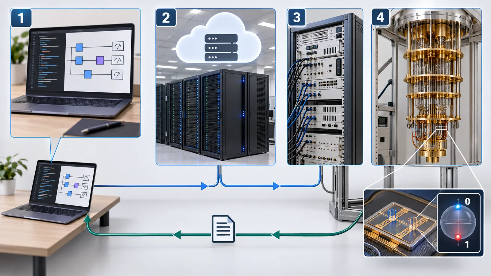
View original SVG, values and sources
Original SVG reference: Concept diagram (vector drawing). A concept diagram of how a quantum computer is used through the cloud. How use is counted follows the official material of IBM and Amazon Braket [Ref. 5, 6]. The flow of an actual service may differ.
Of the eight steps, 1 to 3 and 8 happen on your own classical computer. Steps 4 to 7 are the work of the cloud and the quantum chip. Step 2, "try it small", matters. Real machines are scarce, waiting takes time, and usage is metered (billed), so the standard practice is to check on a local simulator first that the circuit does what you intended (our commentary).
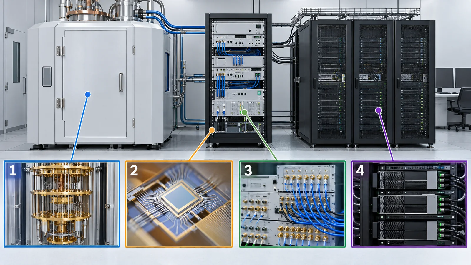
(3) Shots — why we run the same circuit many times
Measuring a qubit gives a probabilistic result. So we run the same circuit N times and count the frequency of each outcome. N is the number of shots. When the probability p of an outcome is estimated from frequencies, a statistical error (the standard error) remains, of size √(p(1−p)/N). Multiplying N by 100 cuts the error to only a tenth.
Statistical fluctuation shrinks, but hardware errors do not. More shots reduce only "chance scatter from too few runs". Errors in gates and measurement, and bias from noise, remain however many times you measure (these are called systematic errors). For example, the small numbers of "01" and "10" that appear in the Bell circuit on real hardware come from hardware errors. Reducing them takes better machines, error mitigation (correcting afterwards in software) and error correction. More shots also lengthen run time and sometimes raise the bill. Amazon Braket, for example, meters quantum computer use by both a "fee per request" and a "fee per shot" [Ref. 6].
(4) Which services, and how they can be used
The table below summarises what we could confirm in official material. Prices change easily, so we give no amounts. We do not rank the services.
| Service | What the official material says (summary) | How use is counted, and plans |
|---|---|---|
| IBM Quantum Platform | A cloud used from Qiskit. Runs through primitives (Estimator and Sampler) [Ref. 3] | Open (free, up to 10 minutes per rolling 28-day window), Flex (pre-purchase of at least 400 minutes, to be used within a year), Pay-As-You-Go, Premium, On-Prem (a dedicated on-premises system) [Ref. 5] Sourced |
| Amazon Braket | Provides quantum computers, circuit simulators, managed hybrid execution and a notebook environment [Ref. 6]. Gate-based devices from AQT, IonQ, IQM and Rigetti, and the analogue device of QuEra, can be used through one framework [Ref. 6] | On demand, a "fee per task" and a "fee per shot", or an hourly reservation (in 1-hour units) [Ref. 6]. The SV1, DM1 and TN1 simulators are billed by run time [Ref. 6]. Hybrid jobs can use PennyLane, CUDA-Q and the Braket SDK [Ref. 6, 7] Sourced |
| Azure Quantum | Microsoft Azure's quantum cloud. Offers real hardware, simulation and estimation of the resources a future large machine would need [Ref. 8]. Its development kit, the QDK, supports Q#, Qiskit, Cirq and OpenQASM [Ref. 8] | Needs an Azure account and a "workspace" [Ref. 8] Sourced |
| Quantinuum | The company's site presents Helios as a hardware service available "on-premises, in the cloud, or both" [Ref. 44] | (details not checked) Sourced |
| IonQ | The company's site presents a "Quantum Cloud" [Ref. 45] | (details not checked) Sourced |
| OQTOPUS (open source) | An operating platform for cloud-based quantum computing systems, developed in Japan [Ref. 26] | — |
Checked 16 October 2026. The summaries rely on each company's official documents and pages. The scope of services, device types and plan names can change. We did not check the terms of use of Quantinuum and IonQ.
(5) IBM's "execution modes": job, batch and session
In work that goes back and forth between quantum and classical computers (Section 6), joining the queue anew each time takes a long time. So IBM's service has three execution modes that differ in how they queue [Ref. 4] Sourced.
| Mode | What the official documentation says (summary) | Suited to (our arrangement) |
|---|---|---|
| Job | A single request sent on its own, not as part of a group | Work that finishes in one run |
| Batch | Several mutually independent jobs are sent together at once. The order of execution is not guaranteed, and they may run in parallel with other users' jobs. The wait for the first job is not shortened | Running many circuits with varied conditions |
| Session | A window in which the system is reserved for a period. During it no other jobs run, and calibration jobs do not run either. Open-plan users cannot submit session jobs | Iterative work where the next circuit depends on the result |
Source: IBM Quantum official documentation (Ref. 4). For what "reserved" means and the details of time limits (TTL), see that document.
A backend is what runs the circuit (real hardware or a simulator). A job is one request sent to it. A primitive is the "type" of request. In Qiskit there are two: Sampler, which measures a circuit many times to get a distribution, and Estimator, which finds the expectation value of an observable (such as energy) [Ref. 3].
Qiskit's documentation explains that the older backend.run has been superseded by primitives (Sampler provides the same direct execution) [Ref. 3] Sourced. This is one reason code in older tutorials may not run on current versions.
6. Hybrid quantum-classical execution
(1) An everyday example: tasting while adjusting the seasoning
When you adjust the flavour of a pot, you taste, add seasoning, and taste again, repeatedly. Here, the taster is the quantum chip and the one deciding how much to add is the classical computer. A method in which a quantum circuit is used for "evaluation", and the classical computer looks at the result and re-sets the circuit's parameters (adjustment knobs inside the circuit), repeating the back-and-forth, is called hybrid (quantum-classical) execution.
The best-known example is the variational quantum eigensolver (VQE). To find the energy of a molecule, a parameterised circuit prepares a "trial state", and its energy expectation value is measured on the quantum chip. The classical computer updates the parameters in the direction that lowers the expectation value, and this repeats. It rests on the idea that the lower the energy expectation, the closer the state is to the true lowest-energy state (the variational principle) (our explanation). Peruzzo and colleagues demonstrated the principle on a photonic quantum processor in 2014 [Ref. 27], and in 2017 Kandala and colleagues found ground-state energies of molecules up to BeH₂ (up to six qubits) on superconducting qubits [Ref. 28] Sourced.
(2) Classical processing next to the quantum chip works on a microsecond scale
Hybrid work has two time worlds.
- Near time (via the cloud): a round trip of sending a circuit and receiving the result takes seconds to minutes or more, including waiting. The back-and-forth of VQE happens in this world
- Real time (within the qubits' coherence time): classical processing that reads a measurement result and decides the next operation before the qubits fall apart. Error-correction decoding and other work that needs microsecond response belong here
The OpenQASM 3 paper builds on exactly this distinction. It says the language was made to handle classical computation in real time, within the qubits' coherence time, and in looser near time, and to allow control flow and calls to external classical functions [Ref. 9] Sourced.
The figures are values stated in each source. One surface-code cycle is about 1.1 μs and the real-time decoder's mean latency is 63 μs (distance 5), as reported in Google's paper [Ref. 31] Sourced. IBM announced decoding of qLDPC codes in real time in under 480 nanoseconds on classical hardware [Ref. 32]. NVIDIA describes NVQLink as having a GPU-to-QPU throughput of 400 Gb/s and a latency of under 4 microseconds, and says that decoding on Quantinuum's Helios had a reaction time of 67 microseconds [Ref. 17]. All of these are company announcements (company claims), and figures that measure different things under different conditions cannot simply be compared.
A qubit's lifetime (coherence time) is limited, and error correction must read a measurement result and decide the next step at once. If the decision is slow, the qubits pile up errors in the meantime.
So designs that place the control electronics (such as FPGAs) and the GPUs or CPUs for decoding right next to the quantum chip, joined by a dedicated high-speed link, are being studied. NVIDIA's blog describes a mechanism called cudaq::device_call that lets a quantum kernel in a CUDA-Q program call GPU or CPU functions directly [Ref. 46].
Link latency, programming language and control hardware become one connected design. The boundary between software and hardware is not fixed (our explanation).
(3) Combining with supercomputers
Raw measurement results from a quantum chip contain noise. So methods are being studied in which measurement results are processed by large classical computations to solve chemistry problems. The work of Robledo-Moreno and colleagues (a method called sample-based quantum diagonalisation, SQD) processed measurement results (quantum samples) from the superconducting processor Heron on the supercomputer Fugaku, and computed the ground states of the dissociation of the nitrogen molecule and of two iron-sulfur clusters ([2Fe-2S] and [4Fe-4S]). It used circuits of up to 77 qubits and 10,570 gates, and says the method gives an upper bound on the ground-state energy [Ref. 29] Sourced. Alexeev and colleagues have also published a perspective paper that organises the idea of "quantum-centric supercomputing", closely integrating quantum and supercomputers, from the viewpoint of materials science [Ref. 30]. In November 2025 IBM announced that it would provide a C API for Qiskit, and a C++ interface built on it, so that quantum computers can be programmed directly from HPC (high-performance computing) environments [Ref. 32] (company description).
It is one possibility, but practical advantage has not been established. The studies above are demonstrations of methods that combine quantum and classical computing. They do not conclude that "a problem classical computers alone cannot solve was solved" (for how to read advantage claims, see "How to Read Quantum Advantage Claims" in this series). In hybrid work the classical part is often large, so take care over "how much of the result is the quantum part's contribution", which can be hard to tell (our explanation).
7. A materials engineer's view — the link to materials computation, and handling data
Why does an article on software have a materials view? There are three reasons. (1) One of the leading intended uses of quantum computers is computation in materials and chemistry. (2) The limit of simulating them on an ordinary classical computer is close to what people in materials computation already feel. (3) Like experimental data, the results of quantum computing need discipline in record-keeping and reproducibility.
The "state-vector method", which simulates a quantum circuit directly on a classical computer, stores the state of n qubits as 2n complex numbers. Counting at double precision (16 bytes each), the memory needed is 16×2n bytes (Our calculation).
Each added qubit doubles the memory: 16 GiB at 30 qubits, 16 TiB at 40 qubits and 16 PiB at 50 qubits (Our calculation). Those with experience in materials computation will recall that as the number of electrons grows, the size of an exact calculation grows exponentially. The expectations for quantum computers rest on the same wall. Robledo-Moreno and colleagues state that on current quantum processors alone, deep circuits and large numbers of measurements make run times prohibitive, and so they demonstrated a way to hand everything except the intrinsically quantum part to classical distributed computing [Ref. 29] Sourced. A realistic picture is not "put the whole material on a quantum computer" but narrow it to the important part as a small problem and process the rest classically (our explanation; see each paper for the actual procedures). However, classical methods that do not use the state-vector method (tensor networks and others) can handle much larger sizes for some circuits. It does not mean that "50 qubits can never be done classically".
You would hardly publish a measurement on a material without recording the sample lot, the instrument and the conditions. Quantum results also need the same discipline, because the same circuit gives different results on a different machine, on a different day, or with different software settings. The items below are our suggestions for what to record (our arrangement; they are not required fields of any service).
| What to record | Why it matters |
|---|---|
| Machine (backend) name and execution date and time | Machines differ in usable gates, connectivity and error size. IBM's documentation says calibration jobs may run in the middle of a batch [Ref. 4], which shows that a machine's state is updated over time |
| Versions of the SDK and transpiler, optimisation level, random seed | The transpiler has stochastic parts. In our example, changing the seed left the number of CZ gates the same but changed the depth (Section 4). New versions improve the algorithms (LightSABRE [Ref. 13]) |
| The converted circuit (saved as OpenQASM 3 or similar) | "The circuit you wrote" and "the circuit actually run" are different things. Saving the latter allows re-running and checking |
| Number of shots and the raw counts (frequencies) | Once boiled down to an expectation value, the statistical error cannot be estimated afterwards (Section 5) |
| Settings of post-processing such as error mitigation | The same measured data gives different results with different post-processing |
| Job ID and plan (shared or reserved) | Needed for enquiries and retrieval. Whether the machine was reserved (session) can change the effect of calibration [Ref. 4] |
Circuits and input data sent to a quantum cloud are also data handed to an external service. If you put a manufacturer's unpublished molecular structure or composition into the circuit parameters, handle it according to your company's data-management rules. IBM's plans include a dedicated on-premises option (On-Prem), described for those who need "high control over their resources and data" [Ref. 5] Sourced.
A transpiler can improve results by reducing the two-qubit gates in a circuit and choosing a placement suited to the machine's state (Section 4). But the error of a single gate is decided by the chip's materials, fabrication, refrigerator and wiring (see "Superconducting Qubits" and "Cryogenics and Control" in this series). Shortening a circuit does not change the error of one gate. Software and hardware (materials) work as a pair (our explanation).
There is one more point of contact close to materials work. PennyLane can compute gradients of variational circuits in a form compatible with machine-learning libraries [Ref. 15] Sourced. This means quantum circuits can be linked with tools from the same Python world as materials data analysis and machine-learned interatomic potentials (our explanation). Moreover, the proposers of OQTOPUS state that opening up the operating platform, as it does, lowers the barrier for research institutions to run their own quantum computing systems [Ref. 26].
8. What could not be confirmed, and a summary
What could not be confirmed
- Measured waiting times (queues) and price amounts: they change easily and depend on conditions, so we give no figures.
- Latest versions of tket, Q# / QDK and the Braket SDK: we checked only Qiskit, Cirq, CUDA-Q and PennyLane on PyPI.
- The licence of the QIR specification and of OQTOPUS: we could not confirm them from GitHub's display (the QIR specification repository shows its licence as undetermined).
- International standardisation of QIR and OpenQASM: we could not confirm any statement that they are ISO or similar standards.
- Terms of use and prices of Quantinuum's and IonQ's cloud services: we confirmed only that the companies' sites present them, and not the details.
- Independent verification of IBM's "decoding in under 480 nanoseconds", of NVIDIA's NVQLink latency and of Quantinuum's decoding time: treated as company announcements; we did not confirm independent verification.
- The public availability of Qiskit's C API and C++ interface as of October 2026: we have only the statement in the November 2025 announcement.
- The latest measured values of each benchmark for each machine: this article concentrates on how to read the metrics and gives no list of values.
- The text of ISO/IEC 4879:2024, and the publication status of IEEE P7131: the text is paid; the publication status could not be confirmed.
- Statistics on SDK user numbers or market share: we could not confirm them, so we do not write "most widely used" or any other ranking.
- A quantum program is a "circuit": a circuit of H, CNOT and measurement is run many times and the frequencies of outcomes are counted. In our run of the Bell circuit, "00" came up 502 times and "11" 498 times Our calculation
- There are several SDKs: Qiskit, Cirq, CUDA-Q, PennyLane and others can all write the same Bell circuit. OpenQASM 3 and QIR serve as common languages for circuits (neither is an ISO or similar standard) Sourced
- The transpiler matters: a 5-qubit QFT went from 56 CZ gates to 30 on a chip with qubits in a line, depending on optimisation strength, and to 20 with full connectivity Our calculation
- Cloud use: send a job, wait in the queue, receive the result. More shots shrinks only statistical fluctuation, not hardware errors Sourced / Our calculation
- Hybrid: there is a near-time (seconds to minutes) back-and-forth and a real-time (microsecond) classical process. Companies are competing to speed up the latter (company claims) Sourced
- For materials engineers: simulator memory doubles with each qubit. Keep records with the discipline of a lab notebook: machine, versions, random seed, shots and the converted circuit Our calculation
9. How to read evaluations and standards
The yardsticks for software and cloud use are: (1) how circuits are written and passed on (the description specifications), (2) the machine's quality, (3) speed, (4) scale and (5) performance on applications. Hardware performance is treated in detail in separate articles ("Coherence and Fidelity" and "How to Read Quantum Advantage Claims"), so here we organise the metrics that are visible from the software and execution side. Check date: 16 October 2026.
| Item evaluated | Representative benchmark or method (name, version and source) | Standards and guidance (ISO/IEC, IEEE and others) | Cautions in reading |
|---|---|---|---|
| How circuits are written, and compatibility | OpenQASM 3: paper (ACM Trans. Quantum Comput. 3, 2022) [Ref. 9], specification v3.1.0 (released 15 May 2024) [Ref. 10]. QIR: the QIR Alliance's specification [Ref. 11] Sourced | We could not confirm that either is an ISO or similar standard. They are specifications managed by communities and companies | The available features differ by specification version. Check that the OpenQASM version your SDK writes matches what the machine accepts |
| Quality (overall) | Quantum volume: a way of validating a machine with randomised circuits (Cross et al., Phys. Rev. A 100, 2019) [Ref. 33]. In a September 2024 blog Quantinuum says its quantum volume has passed two million (company claim) [Ref. 44] Sourced | Could not be confirmed | Quantum volume focuses on the highest-quality part of the machine and is a discrete pass-or-fail metric, so it is said to represent the average quality of a large machine poorly (a point made by McKay et al.) [Ref. 35] |
| Quality (machines at scale) | Layer fidelity and EPLG: the fidelity of a layer of connected two-qubit gates, measured by simultaneous randomised benchmarking (McKay et al., arXiv:2311.05933) [Ref. 35] Sourced | Could not be confirmed | The value changes with which chain of qubits is chosen. We introduce only the idea of the metric and list no values for particular machines |
| Speed | CLOPS (circuit layer operations per second): Wack et al. (2021, arXiv:2110.14108) [Ref. 34]. CLOPS_h: a definition that measures sustained throughput on layered, hardware-aware circuits (Wack, August 2026, arXiv:2608.18044; preprint) [Ref. 38] Sourced | Could not be confirmed | It is meant to measure speed close to the user's experience, including classical processing (conversion and communication). The old CLOPS and CLOPS_h are defined differently, so do not mix them |
| Three metrics (scale, quality, speed) | IBM blog (16 July 2026): programmable qubits, qubit operations and maximum circuits per second [Ref. 40] (company description) | Could not be confirmed | The proposal comes from a machine builder. It is described as applicable to several technologies, but we did not check whether other makers measure by the same definitions |
| Performance on applications | The QED-C application-oriented benchmarks (Lubinski et al., IEEE Trans. Quantum Eng. 4, 2023) [Ref. 36] Sourced | Could not be confirmed | Results are per algorithm and do not reduce to one number. Results can change with the SDK and transpiler settings |
| Computational power (circuit size × speed) | QUOPS (Proctor et al., September 2026, arXiv:2609.12146; preprint): measures the largest computationally meaningful circuit a machine can run successfully and how fast it runs it. Applied to processors from Quantinuum, Google and IBM; it states that about 5 orders of magnitude more capability is needed for useful computation [Ref. 37] Sourced | Could not be confirmed | A preprint, not yet peer reviewed. Results on physical qubits and on logical qubits are mixed, so check which is meant |
| A shared platform and proposals for standardisation | Metriq: an open-source collaborative platform that collects results from several machines (Cosentino et al., March 2026, arXiv:2603.08680) [Ref. 39]. Acuaviva et al.: a proposal toward a standard performance-evaluation approach (Quantum Sci. Technol. 11, 025004, 2026) [Ref. 41] Sourced | At the stage of proposals; not international standards | Check who measured, under what conditions, and whether the data are public |
| Terminology | — (a terminology standard, not an evaluation) | ISO/IEC 4879:2024 "Information technology — Quantum computing — Vocabulary" (published May 2024; the text is paid) [Ref. 42] Sourced | A standard for aligning terms. It does not decide pass or fail for software quality or performance. We have not seen the text |
| Draft standard for performance metrics and benchmarks | — | The site of the IEEE P7131 working group [Ref. 43] Not yet confirmed | At the stage of a draft standard. We could not confirm its publication status |
The arrangement of the table is commentary (ours). The names, sources and dates of each metric were checked against papers and official pages (checked 16 October 2026). The text of standards is paid, so we stay with titles and scope.
Cautions in reading (for materials engineers)
- A "benchmark number" is a value with its conditions: even on the same machine it can change with transpiler settings, software versions and calibration time. Numbers without records cannot be compared (Section 7)
- Look at the relationship between proposer and what is measured: quantum volume, CLOPS and layer fidelity are mainly metrics proposed by IBM researchers [Ref. 33, 34, 35]. Whether other companies use them, and whether independent third parties measure them, must be checked separately
- Separate preprints from peer-reviewed work: CLOPS_h, QUOPS and Metriq are 2026 preprints [Ref. 37, 38, 39]
- Physical qubits or logical qubits: the QUOPS paper has evaluations on both physical qubits and logical qubits [Ref. 37]. The numbers mean entirely different things
- Standards are still at the stage of terminology: ISO/IEC 4879 is a terminology standard with no legal force (in general a standard becomes binding only when cited in law or in a contract; our explanation). Standards for performance metrics are still draft standards such as IEEE P7131, and we could not confirm any established consensus
10. Glossary
- Quantum circuit
- A list of gates and measurements applied to qubits, in order.
- Gate
- An operation that changes the state of qubits, such as H and CNOT.
- Basis gates
- The small set of gates a machine can perform directly. Other gates are broken down into these.
- Measurement
- Reading a qubit out as 0 or 1. The result is decided by probability.
- Shots
- The number of times the same circuit is repeated and measured.
- Standard error
- A guide to the statistical error when estimating a probability from frequencies: √(p(1−p)/N).
- SDK
- Software development kit. A tool for writing circuits and sending them to simulators or real machines.
- Qiskit / Cirq / CUDA-Q / PennyLane
- Leading quantum SDKs. All are open source (Apache-2.0).
- OpenQASM
- An assembly-like language for writing quantum circuits. Version 3 also handles real-time classical processing.
- QIR
- A specification that expresses quantum programs on top of LLVM intermediate representation.
- Transpiler
- A program that rewrites a circuit to fit a machine's gates and connectivity.
- Layout / routing
- The stage that assigns circuit qubits to physical qubits / the stage that connects distant pairs with SWAPs.
- SWAP
- An operation that exchanges the states of two qubits. Equivalent to three CNOTs.
- Circuit depth
- The number of layers when gates that can run in parallel are put in the same layer. A guide to run time.
- NP-hard
- A kind of problem whose cost of an exact solution grows explosively with size.
- QFT
- Quantum Fourier transform. A building block of many quantum algorithms.
- Backend
- What runs a circuit: real hardware or a simulator.
- Job / queue
- One execution request / the waiting line.
- Primitive
- Qiskit's types of request: Sampler (sampling) and Estimator (estimating expectation values).
- Batch / session
- Sending several jobs together / reserving the system for a period (IBM).
- Calibration
- Tuning a machine's operation and measuring its errors. It is updated regularly.
- State-vector method
- Simulating a quantum state on a classical computer by keeping it as 2n numbers.
- Hybrid (quantum-classical)
- Using quantum circuits and classical computation back and forth.
- VQE / SQD
- Variational quantum eigensolver / sample-based quantum diagonalisation. Mixed quantum-classical methods for chemistry problems.
- Real time / near time
- Classical processing within the qubits' coherence time / classical processing on a looser time scale.
- QPU
- Quantum processing unit (the quantum chip).
- Decoding
- Classical processing in error correction that infers where errors occurred from measurement results.
- HPC
- High-performance computing, such as on supercomputers.
- Quantum volume / CLOPS / EPLG
- Benchmarks for a machine's quality / speed / quality at scale (Section 9).
11. References
- Javadi-Abhari A. et al. "Quantum computing with Qiskit", arXiv:2405.08810 (2024) — arxiv.org/abs/2405.08810
- IBM Quantum "Transpiler stages" (Qiskit official documentation; checked 16 October 2026) — quantum.cloud.ibm.com/docs/en/guides/transpiler-stages
- IBM Quantum "Introduction to primitives" (official documentation; checked 16 October 2026) — quantum.cloud.ibm.com/docs/en/guides/primitives
- IBM Quantum "Introduction to Quantum Compute execution modes" (official documentation; checked 16 October 2026) — quantum.cloud.ibm.com/docs/en/guides/execution-modes
- IBM Quantum "Plans overview" (official documentation; checked 16 October 2026) — quantum.cloud.ibm.com/docs/en/guides/plans-overview
- Amazon Web Services "Amazon Braket pricing" (official page; checked 16 October 2026) — aws.amazon.com/braket/pricing/
- Amazon Web Services "What is Amazon Braket?" (official documentation) — docs.aws.amazon.com/braket/…/braket-what-is-Braket.html
- Microsoft "What is Azure Quantum?" (official documentation; checked 16 October 2026) — learn.microsoft.com/…/overview-azure-quantum
- Cross A. et al. "OpenQASM 3: A Broader and Deeper Quantum Assembly Language", ACM Transactions on Quantum Computing 3, 1–50 (2022), DOI 10.1145/3505636 — doi.org/10.1145/3505636
- OpenQASM GitHub repository (specification v3.1.0, 15 May 2024; the official site is openqasm.com; licence Apache-2.0; checked 16 October 2026) — github.com/openqasm/openqasm
- QIR Alliance "Quantum Intermediate Representation" (official site; checked 16 October 2026) — qir-alliance.org
- Li G., Ding Y., Xie Y. "Tackling the Qubit Mapping Problem for NISQ-Era Quantum Devices", ASPLOS '19, 1001–1014 (2019), DOI 10.1145/3297858.3304023 — doi.org/10.1145/3297858.3304023
- Zou H. et al. "LightSABRE: A Lightweight and Enhanced SABRE Algorithm", arXiv:2409.08368 (2024) — arxiv.org/abs/2409.08368
- Sivarajah S. et al. "t|ket⟩: a retargetable compiler for NISQ devices", Quantum Sci. Technol. 6, 014003 (2020), DOI 10.1088/2058-9565/ab8e92 — doi.org/10.1088/2058-9565/ab8e92
- Bergholm V. et al. "PennyLane: Automatic differentiation of hybrid quantum-classical computations", arXiv:1811.04968 (2018) — arxiv.org/abs/1811.04968
- NVIDIA "CUDA-Q" (official documentation; checked 16 October 2026) — nvidia.github.io/cuda-quantum/latest/
- NVIDIA "World's Leading Scientific Supercomputing Centers Adopt NVIDIA NVQLink to Integrate Grace Blackwell Platform With Quantum Processors", press release (17 November 2025) (company announcement) — nvidianews.nvidia.com/news/scientific-supercomputing-centers-nvqlink-…
- Qiskit GitHub repository (licence Apache-2.0; checked 16 October 2026) — github.com/Qiskit/qiskit
- Cirq GitHub repository (Apache-2.0) — github.com/quantumlib/Cirq
- CUDA-Q GitHub repository (Apache-2.0) — github.com/NVIDIA/cuda-quantum
- PennyLane GitHub repository (Apache-2.0) — github.com/PennyLaneAI/pennylane
- tket GitHub repository (under Quantinuum's organisation; Apache-2.0) — github.com/Quantinuum/tket
- Microsoft Quantum Development Kit (Q#) GitHub repository (MIT) — github.com/microsoft/qdk
- Amazon Braket SDK GitHub repository (Apache-2.0) — github.com/amazon-braket/amazon-braket-sdk-python
- PyPI pages of each package (qiskit 2.6.0, cirq 1.7.0, cudaq 0.16.0, pennylane 0.45.1; checked 16 October 2026) — pypi.org/project/qiskit/, pypi.org/project/cirq/, pypi.org/project/cudaq/, pypi.org/project/pennylane/
- Kakuko N. et al. "A Practical Open-Source Software Stack for a Cloud-Based Quantum Computing System" (OQTOPUS), arXiv:2507.23165 (2025); IEEE QCE 2025, DOI 10.1109/QCE65121.2025.00092 — arxiv.org/abs/2507.23165
- Peruzzo A. et al. "A variational eigenvalue solver on a photonic quantum processor", Nature Communications 5, 4213 (2014), DOI 10.1038/ncomms5213 — doi.org/10.1038/ncomms5213
- Kandala A. et al. "Hardware-efficient variational quantum eigensolver for small molecules and quantum magnets", Nature 549, 242–246 (2017), DOI 10.1038/nature23879 — doi.org/10.1038/nature23879
- Robledo-Moreno J. et al. "Chemistry beyond the scale of exact diagonalization on a quantum-centric supercomputer", Science Advances 11, eadu9991 (2025), DOI 10.1126/sciadv.adu9991 (arXiv:2405.05068) — doi.org/10.1126/sciadv.adu9991
- Alexeev Y. et al. "Quantum-centric Supercomputing for Materials Science: A Perspective on Challenges and Future Directions", Future Generation Computer Systems (2024), DOI 10.1016/j.future.2024.04.060 (arXiv:2312.09733) — arxiv.org/abs/2312.09733
- Google Quantum AI and Collaborators "Quantum error correction below the surface code threshold", Nature 638, 920–926 (2025), DOI 10.1038/s41586-024-08449-y (arXiv:2408.13687) — doi.org/10.1038/s41586-024-08449-y
- IBM "IBM Delivers New Quantum Processors, Software, and Algorithm Breakthroughs on Path to Advantage and Fault Tolerance", press release (12 November 2025) (company announcement) — newsroom.ibm.com/2025-11-12-ibm-delivers-new-quantum-processors,->newsroom.ibm.com/2025-11-12-ibm-delivers-new-quantum-processors
- Cross A. W. et al. "Validating quantum computers using randomized model circuits", Phys. Rev. A 100, 032328 (2019), DOI 10.1103/PhysRevA.100.032328 — doi.org/10.1103/PhysRevA.100.032328
- Wack A. et al. "Quality, Speed, and Scale: three key attributes to measure the performance of near-term quantum computers", arXiv:2110.14108 (2021) — arxiv.org/abs/2110.14108
- McKay D. C. et al. "Benchmarking Quantum Processor Performance at Scale", arXiv:2311.05933 (2023) — arxiv.org/abs/2311.05933
- Lubinski T. et al. "Application-Oriented Performance Benchmarks for Quantum Computing", IEEE Transactions on Quantum Engineering 4, 1–32 (2023), DOI 10.1109/TQE.2023.3253761 — doi.org/10.1109/TQE.2023.3253761
- Proctor T. et al. "Benchmarking the computational power of quantum computers", arXiv:2609.12146 (September 2026) (preprint) — arxiv.org/abs/2609.12146
- Wack A. "CLOPS: Benchmarking System Speed at Utility Scale", arXiv:2608.18044 (August 2026) (preprint) — arxiv.org/abs/2608.18044
- Cosentino A. et al. "Metriq: A Collaborative Platform for Benchmarking Quantum Computers", arXiv:2603.08680 (March 2026) (preprint) — arxiv.org/abs/2603.08680
- McKay D. et al. (IBM) "How to measure the performance of a quantum computer", IBM Quantum blog (16 July 2026) (company description) — ibm.com/quantum/blog/hardware-metrics-2026
- Acuaviva A. et al. "Benchmarking quantum computers: towards a standard performance evaluation approach", Quantum Sci. Technol. 11, 025004 (2026), DOI 10.1088/2058-9565/ae4269 — doi.org/10.1088/2058-9565/ae4269
- ISO/IEC 4879:2024 "Information technology — Quantum computing — Vocabulary" (published May 2024). Number, title, date and "Published" status checked on the listing page of the Institute for Standardization of Serbia (ISS) — iss.rs/en/project/show/iso:proj:80432
- IEEE P7131 Working Group "Quantum Benchmarking Working Group P7131" (the working group's site, covering a draft standard for performance metrics and benchmarks of quantum computing) — sagroups.ieee.org/7131
- Quantinuum "Technical perspective: By the end of the decade, we will deliver universal, fully fault-tolerant quantum computing", official blog (September 2024). The site navigation describes how Helios is offered (on-premises or cloud), and the text states a quantum volume above two million — quantinuum.com/blog/technical-perspective…
- IonQ "IonQ roadmap" (official page; the site navigation lists Quantum Cloud; checked 16 October 2026) — ionq.com/roadmap
- NVIDIA "NVIDIA NVQLink Architecture Integrates Accelerated Computing with Quantum Processors", NVIDIA Technical Blog (company description) — developer.nvidia.com/blog/nvidia-nvqlink-architecture-…
12. Claim-to-source audit
| Claim in the text | Basis | Label |
|---|---|---|
| That Qiskit is an SDK for quantum information science covering the representation and optimisation of circuits, support for new gates, mixed quantum-classical computation with dynamic circuits, and the surrounding tools and plugins | Abstract of Javadi-Abhari et al. (2024) Reference 1 https://arxiv.org/abs/2405.08810 | Sourced |
| The six stages of transpiling (init, layout, routing, translation, optimization, scheduling), optimisation levels 0 to 3, and that SabreSwap is stochastic | IBM Quantum official documentation Reference 2 https://quantum.cloud.ibm.com/docs/en/guides/transpiler-stages | Sourced |
| That primitives (Sampler and Estimator) supersede backend.run | IBM Quantum official documentation Reference 3 https://quantum.cloud.ibm.com/docs/en/guides/primitives | Sourced |
| The description of the three execution modes, job, batch and session (batch order is not guaranteed; a session is reserved and calibration jobs also do not run; Open-plan users cannot use sessions) | IBM Quantum official documentation Reference 4 https://quantum.cloud.ibm.com/docs/en/guides/execution-modes | Sourced |
| IBM's plans (Open: up to 10 minutes per rolling 28-day window; Flex: pre-purchase of at least 400 minutes; Pay-As-You-Go; Premium; On-Prem: a dedicated on-premises system) | IBM Quantum official documentation Reference 5 https://quantum.cloud.ibm.com/docs/en/guides/plans-overview | Sourced |
| How Amazon Braket prices use (a fee per task plus a fee per shot, or an hourly reservation; the SV1, DM1 and TN1 simulators; hybrid jobs; devices from AQT, IonQ, IQM, Rigetti and QuEra; IonQ error mitigation needs at least 2,500 shots per task) | The AWS pricing page Reference 6 https://aws.amazon.com/braket/pricing/ Reference 7 https://docs.aws.amazon.com/braket/latest/developerguide/braket-what-is-Braket.html | Sourced |
| That Azure Quantum offers real hardware, simulation and resource estimation, and that the QDK supports Q#, Qiskit, Cirq and OpenQASM and is free and open source | Microsoft official documentation Reference 8 https://learn.microsoft.com/en-us/azure/quantum/overview-azure-quantum | Sourced |
| That OpenQASM 3 handles real-time and near-time classical computation, control flow and calls to external classical functions. Specification v3.1.0 (15 May 2024) | Cross et al. (2022); the official GitHub repository Reference 9 https://doi.org/10.1145/3505636 Reference 10 https://github.com/openqasm/openqasm | Sourced |
| That QIR is a specification expressing quantum programs on LLVM intermediate representation, developed by the QIR Alliance | The QIR Alliance's official site Reference 11 https://www.qir-alliance.org/ | Sourced |
| The proposal of SABRE (stochastic qubit placement and routing). The report that LightSABRE is about 200 times faster and cut SWAPs by an average of 18.9% (the authors' report). That tket is a compiler that does not depend on a particular machine | Abstracts of Li et al. (2019) and Zou et al. (2024), title of Sivarajah et al. (2020) Reference 12 https://doi.org/10.1145/3297858.3304023 Reference 13 https://arxiv.org/abs/2409.08368 Reference 14 https://doi.org/10.1088/2058-9565/ab8e92 | Sourced |
| That PennyLane can compute gradients of variational circuits in a form compatible with backpropagation in machine learning, and has plugins for hardware | Abstract of Bergholm et al. (2018) Reference 15 https://arxiv.org/abs/1811.04968 | Sourced |
| That CUDA-Q is a programming model for mixed quantum-classical work. NVQLink's GPU-to-QPU throughput of 400 Gb/s, latency under 4 microseconds, and Quantinuum's decoding reaction time of 67 microseconds on Helios (company announcements). The description of cudaq::device_call | NVIDIA's documentation, press release and technical blog Reference 16 https://nvidia.github.io/cuda-quantum/latest/ Reference 17 https://nvidianews.nvidia.com/news/scientific-supercomputing-centers-nvqlink-grace-blackwell-quantum-processors Reference 46 https://developer.nvidia.com/blog/nvidia-nvqlink-architecture-integrates-accelerated-computing-with-quantum-processors/ | Sourced |
| That the licences of Qiskit, Cirq, CUDA-Q, PennyLane, tket and the Braket SDK are Apache-2.0 and that of Microsoft's QDK is MIT | The display of each GitHub repository (checked 16 October 2026) Reference 18 https://github.com/Qiskit/qiskit Reference 19 https://github.com/quantumlib/Cirq Reference 20 https://github.com/NVIDIA/cuda-quantum Reference 21 https://github.com/PennyLaneAI/pennylane Reference 22 https://github.com/Quantinuum/tket Reference 23 https://github.com/microsoft/qdk Reference 24 https://github.com/amazon-braket/amazon-braket-sdk-python | Sourced |
| The latest PyPI versions on 16 October 2026 (Qiskit 2.6.0, Cirq 1.7.0, CUDA-Q 0.16.0, PennyLane 0.45.1) | The PyPI pages Reference 25 https://pypi.org/project/qiskit/ | Sourced |
| That OQTOPUS is an operating platform for cloud-based quantum computing systems, implements a transpiler, multiprogramming and error mitigation, and is public on GitHub | Abstract of Kakuko et al. (2025) Reference 26 https://arxiv.org/abs/2507.23165 | Sourced |
| VQE demonstrated on a photonic processor in 2014, and in 2017 ground-state energies of molecules up to BeH₂ (up to six qubits) found on superconducting qubits | Peruzzo et al. (2014) and Kandala et al. (2017) Reference 27 https://doi.org/10.1038/ncomms5213 Reference 28 https://doi.org/10.1038/nature23879 | Sourced |
| With Heron and Fugaku, the dissociation of N₂ and the [2Fe-2S] and [4Fe-4S] clusters computed with circuits of up to 77 qubits and 10,570 gates; the method gives an upper bound on the ground-state energy; quantum processors alone have prohibitive run times with deep circuits and many measurements. The perspective on quantum-centric supercomputing in materials science | Abstracts of Robledo-Moreno et al. (2025) and Alexeev et al. (2024) Reference 29 https://doi.org/10.1126/sciadv.adu9991 Reference 30 https://arxiv.org/abs/2312.09733 | Sourced |
| A surface-code cycle of about 1.1 μs and a real-time decoder mean latency of 63 μs (distance 5) | Google (2025) Reference 31 https://doi.org/10.1038/s41586-024-08449-y | Sourced |
| IBM's announcement of real-time decoding of qLDPC codes in under 480 nanoseconds, and of a C API and a C++ interface for Qiskit (November 2025) (company announcement) | IBM press release Reference 32 https://newsroom.ibm.com/2025-11-12-ibm-delivers-new-quantum-processors,-software,-and-algorithm-breakthroughs-on-path-to-advantage-and-fault-tolerance | Sourced |
| The proposals of quantum volume, CLOPS (2021), layer fidelity and EPLG, and the QED-C application-oriented benchmarks | Cross et al. (2019), Wack et al. (2021), McKay et al. (2023), Lubinski et al. (2023) Reference 33 https://doi.org/10.1103/PhysRevA.100.032328 Reference 34 https://arxiv.org/abs/2110.14108 Reference 35 https://arxiv.org/abs/2311.05933 Reference 36 https://doi.org/10.1109/TQE.2023.3253761 | Sourced |
| QUOPS (applied to Quantinuum, Google and IBM; the conclusion that about 5 orders of magnitude more capability is needed; evaluation on up to eight [[7,1,3]] logical qubits of Helios-1), CLOPS_h, Metriq, IBM's three metrics, and the proposal of Acuaviva et al. | The respective preprints, blog and paper Reference 37 https://arxiv.org/abs/2609.12146 Reference 38 https://arxiv.org/abs/2608.18044 Reference 39 https://arxiv.org/abs/2603.08680 Reference 40 https://www.ibm.com/quantum/blog/hardware-metrics-2026 Reference 41 https://doi.org/10.1088/2058-9565/ae4269 | Sourced |
| That ISO/IEC 4879:2024 "Information technology — Quantum computing — Vocabulary" was published in May 2024 | The listing page of the Institute for Standardization of Serbia (ISS) Reference 42 https://iss.rs/en/project/show/iso:proj:80432 | Sourced |
| That the IEEE P7131 working group has a draft standard for performance metrics and benchmarks of quantum computing within its scope. We could not confirm the publication status | The working group's site Reference 43 https://sagroups.ieee.org/7131 | Not yet confirmed |
| That Quantinuum presents Helios as available on-premises, in the cloud, or both; the statement of a quantum volume above two million (company claim). That IonQ's site presents a Quantum Cloud | The companies' official pages Reference 44 https://www.quantinuum.com/blog/technical-perspective-by-the-end-of-the-decade-we-will-deliver-universal-fault-tolerant-quantum-computing Reference 45 https://www.ionq.com/roadmap | Sourced |
| The Bell-circuit results (Qiskit: "00" 502 times and "11" 498 times; Cirq: 512 and 488; CUDA-Q: 499 and 501; PennyLane: 502 and 498; random seed 7, 1000 shots) and the OpenQASM 3 output. The conversion results for the 5-qubit QFT (before conversion: p 30, cx 26, u 5, depth 34. Line: level 0 gives 56 CZ and depth 194, level 1 gives 50 and 123, levels 2 and 3 give 30 and 82; full connectivity at level 3 gives 20 and 56; over seeds 0 to 19 the CZ count was constant and the level-1 depth was 120 to 130). The standard errors (±5% at 100 shots, 1.6% at 1000, 0.5% at 10⁴, 0.16% at 10⁵, 0.05% at 10⁶). The state-vector memory (16×2ⁿ bytes: 16 MiB at 20 qubits, 16 GiB at 30, 16 TiB at 40, 16 PiB at 50) | Our own calculation (Python 3, Qiskit 2.6.0, Cirq 1.7.0, CUDA-Q 0.16.0, PennyLane 0.45.1; local simulators; assumptions stated in the text). Not results from real hardware | Our calculation |
| Waiting times and price amounts, the latest versions of tket, QDK and the Braket SDK, the licences of QIR and OQTOPUS, international standardisation of QIR and OpenQASM, the terms of use of Quantinuum and IonQ, independent verification of the latency and speed claims, the public availability of Qiskit's C API as of October 2026, the latest benchmark values for each machine, the text of ISO/IEC 4879, the publication status of IEEE P7131, and SDK user numbers or market share | Could not be confirmed in the primary material this article could access, so they are not stated | Commentary |
| The analogies ("a score and a performance", "a shared facility", "tasting while adjusting the seasoning", "deliveries in a town with few direct roads"), the materials-view readings (similarity to the dimension wall, the lab-notebook discipline of records, software and hardware as a pair, the example record items), and the cautions on reading benchmarks | Our own arrangement and explanation based on published material. Not views stated by any of the organisations | Commentary |
| That Fig. 1 and Fig. 7 are ImageGen-generated conceptual illustrations, and that the other figures are explanatory drawings and not observations of real data | A note in this article | Commentary |
Last updated 16 October 2026. Sources are limited to primary material (official documentation, peer-reviewed papers, arXiv papers, public GitHub and PyPI information, official pages of the companies, and the listing page of an ISO standard). Company announcements and plans are kept separate. Software versions, service plans and prices change often. The results of code and numerical estimates are our own calculations on local simulators, not results from real hardware. Waiting times and price amounts, the latest versions of some SDKs, the licences of QIR and OQTOPUS, the state of international standardisation, the terms of use of Quantinuum and IonQ, independent verification of company speed claims, the public availability of Qiskit's C API, the latest benchmark values for each machine, the text of ISO/IEC 4879, the publication status of IEEE P7131 and SDK user numbers could not be confirmed and are not stated here. All figures are explanatory concept diagrams or drawings that include our calculations; Fig. 1 and Fig. 7 are ImageGen-generated conceptual illustrations.