Quantum Algorithms Explained

TECHNOLOGY EXPLAINER

Quantum Algorithms
— Why quantum can be faster: interference, Deutsch, Grover, Shor, phase estimation and simulation

A quantum computer can solve some problems faster, but not "because it computes every answer at once". It is because the computation is designed so that the waves of the right answer reinforce and those of wrong answers cancel. This article assumes no physics background. With figures and small numerical examples it explains this "interference design" pattern through Deutsch's problem (the smallest example), Grover search, Shor factoring, phase estimation and quantum simulation, in that order. The second half covers which problems speed up and which do not, the difference between theory and real machines, and what quantum simulation looks like to a materials engineer. It is the article to read after "Quantum Computing Fundamentals", "Quantum Gates and Quantum Circuits" and "Coherence and Fidelity".

Sources: surveys (Montanaro, Dalzell et al.), peer-reviewed papers (Physical Review, Nature, Science, SIAM J. Comput. and others), arXiv papers, the Quantum Algorithm Zoo, official NIST, DARPA, ISO and IEEE pages / numerical examples are our own calculations / checked on 16 October 2026

**Fig. 1. Conceptual illustration generated with ImageGen.** A scene of thinking about a quantum algorithm with a picture of wave interference and a circuit diagram. It does not depict any real laboratory or document. Not an actual product, facility, dimensional specification or measurement. Distinguish enlarged models from full-scale scenes.

In this article

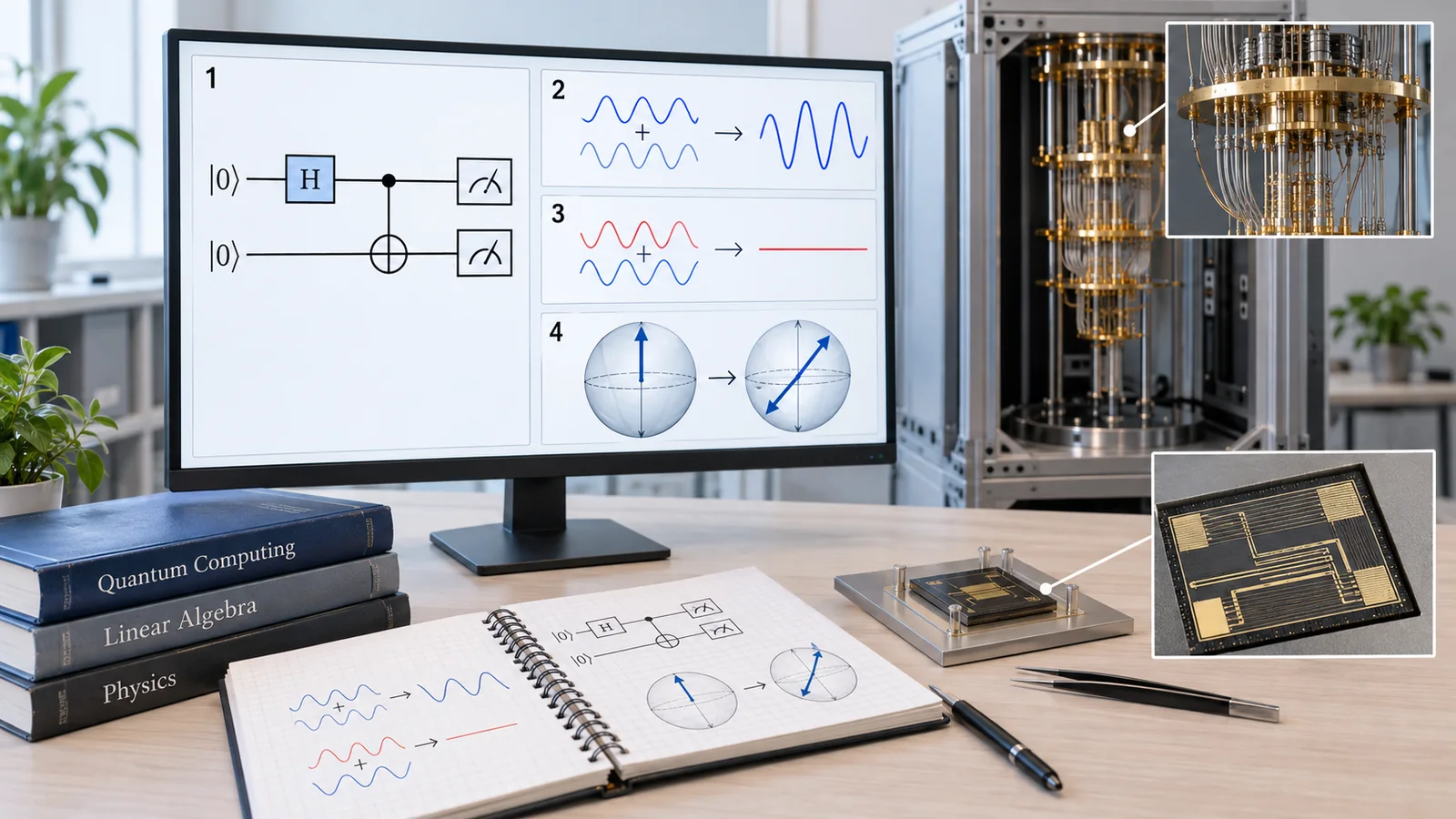
Three-line summary / what to know first / where this sits in the series
Why can it be faster? The answer is "interference"
The smallest example: Deutsch's problem (and Deutsch–Jozsa)
Grover search: a "square-root" speed-up
Shor factoring: finding the "period"
Quantum phase estimation: reading a "rotation speed"
Quantum simulation: Feynman's idea
Which problems speed up, and which do not
Theory versus real machines
A materials engineer's view: what algorithms demand of materials and machines
How to read evaluations and standards
Glossary
References (primary sources)
Claim-to-source audit

Notation used in this article

Sourced = stated in a published source (link given)
Our calculation = a value this article computed or checked from stated assumptions
Not yet confirmed = resource estimates, company and national plans, standards under development and other items that are not settled
Our own reading for materials engineers is marked as commentary; inference is shown in bold. Every analogy comes with a note on where the analogy breaks down.

The numbers in this article, and cryptography

The amplitudes, probabilities, counts and periods in Chapters 3 to 6 are our own illustrative calculations, not measurements from a real device. The resource estimates in Chapter 9 are theoretical estimates under assumptions, not forecasts. We explain Shor's algorithm only as an idea and give no concrete procedure or implementation for breaking encryption. Taking it as given that "when a quantum computer might break encryption" cannot be predicted with confidence, we confine ourselves to describing standards and guidance (Chapter 11). For standards (NIST, ISO/IEC, IEEE) we confirmed only the title and status, not the text. This field moves fast, so statuses carry a check date (16 October 2026).

1. Three-line summary / what to know first / where this sits in the series

The reason is "interference": a quantum algorithm prepares waves, puts the structure of the problem into their signs, uses interference to reinforce the right answer, and measures. It does not "compute all answers at once" Sourced [Refs. 1, 2]
Only a limited set of problems speed up, and by different amounts: factoring (Shor) is faster by a huge margin in theory, while search (Grover) only reduces the count to a "square root". For most problems no quantum speed-up has been shown Sourced [Refs. 3, 4]
Theory and real machines are separate stories: theoretical speed-ups assume a large error-corrected machine. Real demonstrations are small, and the scales estimated to be needed are orders of magnitude beyond today's experimental machines Sourced / Not yet confirmed [Refs. 6, 5]

What to know before reading

We use the arrow, measurement and interference (adding waves, where positive and negative amplitudes can cancel) from "Quantum Computing Fundamentals", and the gates (H, CNOT and others) from "Quantum Gates and Quantum Circuits". If you have not read them, the necessary parts are briefly explained again. Formulas are kept to a minimum, and harder material is tucked into folded "More detail" sections.

Where this sits in the series

This is the article to read after "Coherence and Fidelity", and the last of the four introductory articles of the Quantum Computing series. Error correction, NISQ and hybrid computing, how to read quantum-advantage claims, quantum chemistry and post-quantum cryptography are covered in their own articles in the series.

2. Why can it be faster? The answer is "interference"

When people explain the speed of quantum computers they often say "parallel computation": "a qubit takes 0 and 1 at the same time, so many calculations can be done at once". As the Fundamentals article showed, this wording is a source of misunderstanding. A measurement extracts only one result, and without some design what comes out is just one random candidate.

So what produces the speed? Cleve and colleagues state that the common pattern of quantum algorithms is using quantum interference of several computational paths to enhance correct outcomes and suppress wrong ones Sourced [Ref. 1]. The figure shows this pattern.

Fig. 2 Conceptual diagram (vector drawing). A conceptual diagram of the four-stage pattern common to quantum algorithms. Cleve et al. describe quantum computation as using interference of computational paths to enhance correct outcomes and suppress erroneous ones [Ref. 1].

Common misconception: "quantum computers are fast because they compute in parallel" is inaccurate

A quantum algorithm does not "compute all candidates at once". It assigns waves to all the candidates and makes those waves interfere so that they gather on the right answer. This gathering can be designed well only when the problem has structure that can be used (a period, a symmetry, a mark on the answer). That is why only a limited set of problems speed up (Chapter 8).

A stumbling block: what does "put the structure of the problem into the sign of the waves" mean?

Suppose you want to find a winning candidate. Using a box that checks whether a candidate wins (an oracle), you flip only the sign of the winner's wave (step 2 in the figure). The sign difference does not show up in a measurement as it is, but the next interference turns it into a difference in strength. This is the same mechanism as in the gates article, where Z's "invisible change" becomes visible when sandwiched between H gates (our commentary).

3. The smallest example: Deutsch's problem (and Deutsch–Jozsa)

Let us test the interference pattern on the smallest example. It is a problem proposed by Deutsch in 1985, the first example showing that a quantum computer can answer with fewer queries than a classical one Sourced [Refs. 7, 3].

There is a box f that returns 0 or 1 for an input of 0 or 1. You want to know only whether f(0) and f(1) are the same (constant) or different (balanced). Classically you must ask for both f(0) and f(1), two queries. On a quantum computer, applying H, the oracle and H once gives the answer.

Fig. 3 Chart including our calculation (vector drawing). The circuit and result table for Deutsch's problem (phase-oracle version). The amplitudes are our calculation, checked by matrices for all four functions. The classical-side assessment of Deutsch–Jozsa follows the Quantum Algorithm Zoo [Ref. 3] and Cleve et al. [Ref. 1].

Why does it work? The first H creates waves of equal height (0.71 each) on 0 and 1. The oracle flips the sign of each wave according to the value of f. When the second H adds the two waves, if f is constant they reinforce at "0"; if balanced they cancel at "0". It is the "apply H twice and return" of the Fundamentals article with a sign flip in between. For all four functions, we checked by matrix calculation that the amplitude of "0" is +1 or −1 (constant) or 0 (balanced) Our calculation.

Common misconception: "Deutsch–Jozsa is evidence of an exponential quantum speed-up" is inaccurate

Even for the n-bit Deutsch–Jozsa problem (Deutsch and Jozsa, 1992), one quantum query suffices [Ref. 8]. A classical deterministic method (one that uses no random numbers) needs up to 2ⁿ⁻¹ + 1 queries in the worst case: 524,289 for n = 20. But a classical method that uses random numbers can tell the cases apart with high probability using few queries. The Quantum Algorithm Zoo describes the problem as "probabilistically easy to solve with O(1) queries" and lists the speed-up as "exponential over deterministic classical, none over probabilistic classical" Sourced [Ref. 3]. In our calculation, with n = 20 the error after 10 queries is about 0.195% Our calculation (close to 2¹⁻¹⁰, the chance that a balanced function looks the same on all 10 queries). So the exponential gap holds only against deterministic classical methods and is not proof of practical speed. The "oracle" is a convention that counts a box with unknown contents as one query; the cost of building the box is separate.

A stumbling block: why use a problem that is of no practical use?

Deutsch's problem is not useful in itself. It is a teaching example showing, as small as possible, the mechanism of using interference to pick out an answer. Simon's problem (Simon, 1997) and the Bernstein–Vazirani problem (Bernstein and Vazirani, 1997) follow the same pattern and are also oracle problems Sourced [Refs. 9, 10]. They led to the ideas behind Shor's algorithm (our commentary).

4. Grover search: a "square-root" speed-up

Grover's search (1996) addresses "find the one winner among N candidates", where an oracle can check whether a candidate wins. Classically it takes N/2 queries on average and N in the worst case. Grover's algorithm finds it in about √N queries Sourced [Refs. 11, 3]. The mechanism is the repeated "reflection" below.

Fig. 4 Chart including our calculation (vector drawing). The amplitudes at each stage of Grover search with N = 8, followed by matrix arithmetic (our calculation). The winner's amplitude goes 0.35 → 0.88 → 0.97 → 0.57 and its probability 12.5% → 78.1% → 94.5% → 33.0%. Not a result from a real device. The mechanism follows Grover's paper [Ref. 11].

Take eight candidates (N = 8) with one winner; we followed the amplitudes by matrix calculation. At first all waves have the same height (0.35) and the winner's probability is 12.5% (= 1/8). After one reflection the winner's amplitude is 0.88 (probability 78.1%), after two it is 0.97 (94.5%), and after three it overshoots and falls to 0.57 (33.0%) Our calculation. So more steps are not better; there is a best number, about (π/4)·√N.

Fig. 5 Chart including our calculation (vector drawing). Grover steps versus success probability (N = 8 and 64), and the comparison with the classical average count (N/2) (our calculation). The count is close to (π/4)√N: 785 for N = 10⁶ and 24,836 for N = 10⁹. That the Grover count is optimal (Ω(√N)) was shown by Bennett et al., Zalka and Boyer et al. [Refs. 4, 13, 12].

Number of candidates N	Classical queries (average) N/2	Best Grover steps (about (π/4)√N)	Success probability then
8	4	2	94.5%
64	32	6	99.7%
1,000	500	24	99.96%
10⁶	500,000	785	about 100%
10⁹	500,000,000	24,836	about 100%

Our calculation. We computed Grover's success probability sin²((2k+1)θ) with θ = arcsin(1/√N) and the best number of steps. The classical average was taken as N/2 queries. These are not results from a real device.

That this "square root" is optimal (it cannot be reduced further) was shown by Bennett et al. (1997), Boyer et al. (1998) and Zalka (1999) Sourced [Refs. 4, 12, 13]. For "search with no structure", a quantum computer can reduce the number of tries only to the square root of brute force.

Common misconception: "Grover makes database (web) search instant" is wrong

The name "database search" misleads. Grover's problem is searching among structureless candidates with a box (an oracle) that checks whether a candidate wins. It is not about large, well-organised data such as web search, and it is not "instant" (the count merely becomes √N). The cost of loading data into a quantum state (the input problem) and the cost of running the oracle at each step are separate (our commentary).

A stumbling block: a quadratic speed-up can fail to "pay off" because of error-correction cost

Even if the count drops to √N, if each step is very heavy because of error correction, the total time can be longer than classical brute force. Babbush and colleagues computed that a small polynomial speed-up has trouble making up for the large constant-factor overhead of error correction while the computation must still finish in reasonable time. They conclude that quadratic speed-ups will not enable quantum advantage on early generations of fault-tolerant devices unless the way error correction is realised improves significantly (and say quartic speed-ups look significantly more practical) Sourced [Ref. 14].

5. Shor factoring: finding the "period"

Shor's algorithm (1997) factors large integers into primes in polynomial time on a quantum computer Sourced [Ref. 15]. Factoring means turning a product of primes (for example 15 = 3 × 5) back into the primes, and it gets steeply harder classically as the number grows. According to the Quantum Algorithm Zoo, Shor's algorithm factors an n-bit integer in roughly n³ time (Õ(n³)), while the fastest known classical method (the general number field sieve) is believed to take about 2^{Õ(n^1/3)} time Sourced [Ref. 3].

(1) The idea: turn factoring into "finding a period"

The heart of Shor's algorithm is to restate factoring as the problem of finding a period. Take a small example, N = 15. Pick a = 7 and list the remainder of 7^x divided by 15 for x = 0, 1, 2, …: 1, 7, 4, 13, 1, 7, 4, 13, 1 … The same pattern repeats every 4 terms. That "4" is the period r. Once the period is known, the greatest common divisors of a^r/2 ± 1 with 15 give the factors (the gcd of 49 − 1 = 48 with 15 is 3, and of 49 + 1 = 50 with 15 is 5) Our calculation.

Fig. 6 Chart including our calculation (vector drawing). Shor's idea followed with N = 15 and a = 7 (our calculation: period 4 of 7ˣ mod 15; a 64-point Fourier transform gives peaks of 25% each at 0, 16, 32, 48; gcd(48,15) = 3, gcd(50,15) = 5). The mechanism follows Shor's paper [Ref. 15].

(2) The quantum computer handles only "finding the period"

Quantum interference is used in the part that finds the period. The sequence of remainders is prepared as a "quantum state" and a quantum Fourier transform (a transform that turns a periodic pattern into frequencies) is applied; the waves then reinforce and gather at values tied to the period. In the example in the figure (period 4, 64-point transform), the measured value is only ever 0, 16, 32 or 48 (25% each), and their spacing 16 = 64 ÷ 4 reveals the period 4 Our calculation. If the period does not divide evenly the peaks blur slightly but still gather near certain values, from which the period can be estimated (our calculation: for N = 21, a = 2, period 6 with a 128-point transform, the peaks gather around 0, 21, 43, 64, 85 and 107).

A stumbling block: how "period" and "interference" are related

When waves of a periodic pattern are added, they reinforce only at the frequency that matches the period and cancel elsewhere. It is the same kind of interference as the "beats" of sound, or light strengthening only in certain directions from a diffraction grating. Where the analogy breaks down: a real quantum Fourier transform is a sequence of quantum gates acting on amplitudes, not sound or light themselves (our commentary).

Common misconception: "Shor's algorithm has factored large numbers on a real machine" is wrong

The first demonstration was the factoring of N = 15 by Vandersypen and colleagues (2001), who used seven nuclear spins in a molecule, manipulated by nuclear magnetic resonance. The paper itself says that the method is in principle scalable but that this experiment does not imply it Sourced [Ref. 16]. Smolin and colleagues (2013) then pointed out that many small demonstrations used simplifications that depended on knowing the factors in advance, and that the right measure of difficulty in implementing Shor's algorithm is not the size of the number factored but the length of the period found Sourced [Ref. 17]. A demonstration of "15 = 3 × 5" does not mean practical scale has been reached.

6. Quantum phase estimation: reading a "rotation speed"

The generalisation of Shor's period finding is quantum phase estimation. Kitaev (1995) formulated it, and Cleve and colleagues (1998) showed that many quantum algorithms can be understood as different cases of phase estimation Sourced [Refs. 18, 1].

As an analogy, it is a way of measuring how fast a clock hand turns by stacking many revolutions, so as to read it precisely. When an operation U is applied, a particular state (an eigenstate) changes only in the heading of its arrow. Using n readout qubits and interference, the angle of that rotation (the phase φ) is read out as an n-digit binary number.

Fig. 7 Chart including our calculation (vector drawing). The shape of the phase-estimation circuit and the probability distribution when reading the phase 1/3 with 4 bits (our calculation). Phase estimation was formulated by Kitaev [Ref. 18] and Cleve et al. [Ref. 1]. The circuit is conceptual.

A phase that can be written exactly in two bits, such as φ = 0.25 (binary 0.01), is read with certainty. A phase that cannot be written exactly, such as φ = 1/3, reads out, with four bits, as one of two nearby values. In our calculation y = 5 (estimated phase 0.3125) came out with 68.5% and y = 6 (0.375) with 17.2%; the total probability of falling within 1/16 of the true value was 85.7% Our calculation. Each extra readout qubit doubles the precision.

Phase estimation is a shared component of Shor's algorithm (where the period appears as a phase) and of quantum simulation in the next chapter (where the energy appears as a phase).

7. Quantum simulation: Feynman's idea

In 1982 Feynman pointed out that following a quantum system on a classical computer gets very costly as the system grows, and put forward the idea that a quantum system is naturally imitated by quantum parts Sourced [Ref. 19]. Lloyd (1996) showed that this is actually possible (a universal quantum simulator) Sourced [Ref. 20]. Aspuru-Guzik and colleagues (2005) proposed a way to obtain molecular energies by quantum computation Sourced [Ref. 21].

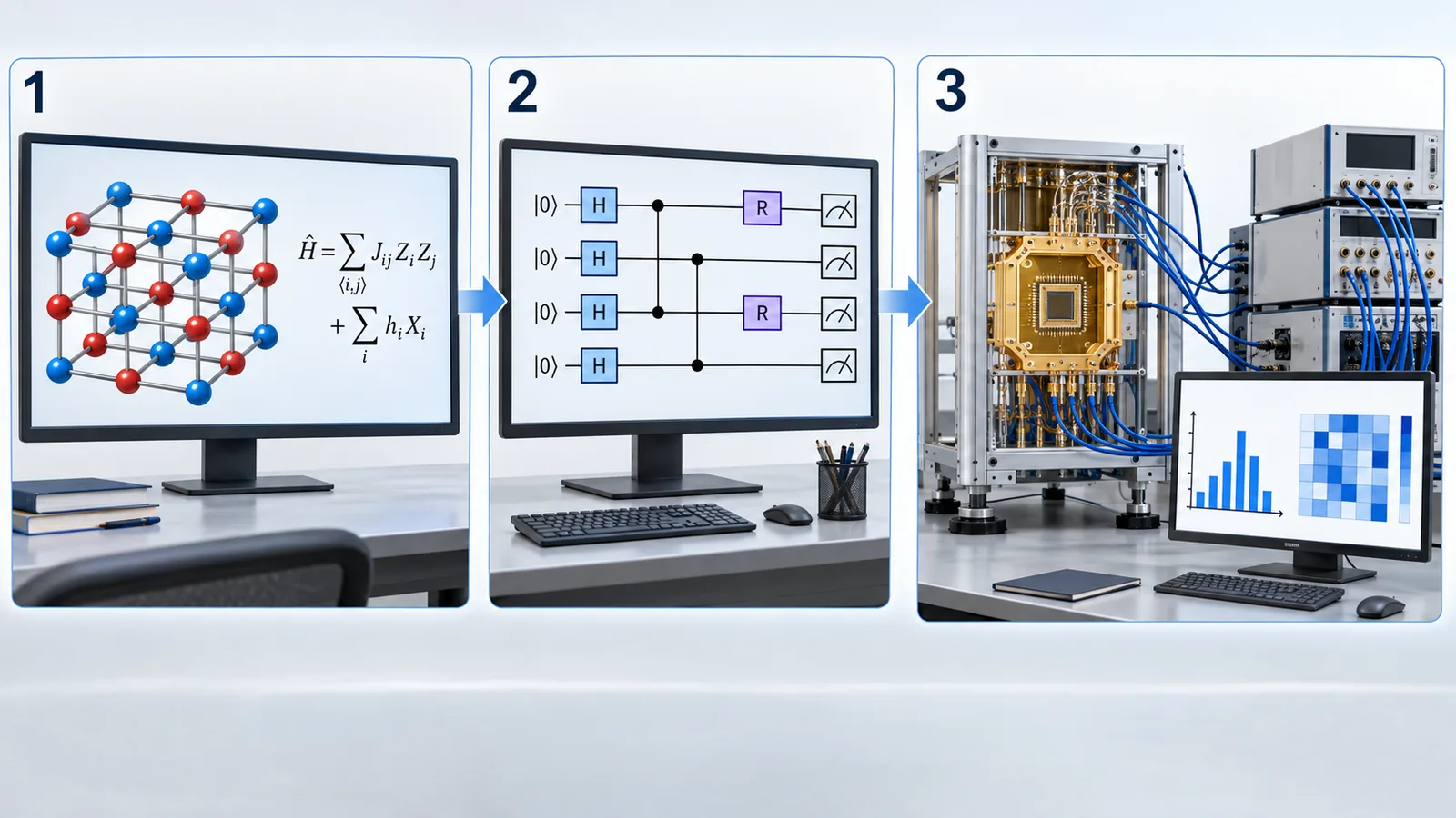
**Fig. 8. Conceptual illustration generated with ImageGen.** A physical-system model is turned into a circuit, quantum measurements are obtained, and classical analysis follows. This does not imply a speedup for every problem. Not an actual product, facility, dimensional specification or measurement. Distinguish enlarged models from full-scale scenes.

View original SVG, values and sources

Original SVG reference: Conceptual diagram (vector drawing). A conceptual diagram of the flow of quantum simulation and how to judge it. Machine examples are from Kandala et al. [Ref. 22] and Xue et al. [Ref. 23], resource estimates from Reiher et al. [Ref. 24] and Lee et al. [Ref. 25], and the assessment from Lee et al. [Ref. 26].

The flow is: describe a molecule or material by an "energy operator (Hamiltonian)", break its time evolution into a sequence of gates, and read out the energy by phase estimation (or a variational method). In quantum chemistry the ground-state energy bears on how readily a reaction proceeds, how a catalyst works and the voltage of a battery material (our commentary).

What machines have done, resource estimates, and assessment

Machines: Kandala and colleagues (2017) used a superconducting quantum processor (up to six qubits) to compute, variationally, small molecules such as lithium hydride and beryllium hydride and a small magnet model Sourced [Ref. 22]. The silicon-spin machine of Xue et al. (2022) also computed a molecular ground-state energy variationally Sourced [Ref. 23]. All are small-scale examples
Resource estimates: Reiher and colleagues (2017) gave resource estimates for studying a reaction mechanism on a quantum computer, using the nitrogen-fixing enzyme (FeMoco) as an example, and Lee and colleagues (2021) showed a way to cut the resources with tensor hypercontraction Sourced [Refs. 24, 25]. These are theoretical estimates, not machine results (Not yet confirmed)
Assessment: Lee and colleagues (2023) conclude that evidence for an exponential quantum advantage across chemistry for ground-state energies has not yet been found (although polynomial speed-ups are possible) Sourced [Ref. 26]. The decider is comparison with the best classical methods (density-functional theory, coupled cluster, tensor-network methods and so on)

A stumbling block: "simulation" is not a model inside the computer, but...

An ordinary "simulation" writes a phenomenon as equations and calculates it on a computer. In quantum simulation, the parts doing the computation are themselves quantum systems, and the behaviour of one system is reproduced with a similar quantum system. Where the analogy breaks down: not every quantum system can be imitated quickly on a quantum computer; the advantage depends on the nature of the problem (whether classical approximations work) (our commentary; see our article on quantum chemistry and materials simulation).

8. Which problems speed up, and which do not

The examples so far let us sort quantum speed-ups by kind. Montanaro's survey organises quantum algorithms by the size of the speed-up (exponential, quadratic, small polynomial and so on) Sourced [Ref. 2]. The survey by Dalzell and colleagues organises each application together with its technical caveats (such as the overall complexity including error correction) Sourced [Ref. 27].

Fig. 9 Conceptual diagram (vector drawing). A map of kinds of quantum speed-up and the state of confirmation of their practicality (conceptual). Each speed-up is a theoretical or "oracle" assessment, not a practical speed-up confirmed on machines.

Kind of problem	Kind of speed-up (in theory)	Caveat
Factoring and discrete logarithms (Shor)	Superpolynomial (by a huge margin over the best known classical method) [3]	Practical scale needs a large error-corrected machine (Chapter 9)
Simulating quantum systems	Problem-dependent. Polynomial speed-ups are expected, but evidence for an exponential advantage across chemistry is not confirmed [26]	Comparison with the best classical methods decides
Unstructured search (Grover)	Quadratic (√N). Cannot be reduced further [13, 4]	Error-correction overhead may erase the gain [14]
General hard problems (NP-complete and so on)	Against an oracle, at best the square root of brute force (cannot go below 2^n/2) [4]	Whether all of NP can be solved in quantum polynomial time is an open question
Linear equations and machine learning (HHL and others)	Superpolynomial under conditions (Harrow et al., 2009) [28]	Aaronson says details (loading the input, reading the output, the condition number) must be checked [29]. Tang (2019) matched the speed classically for a recommendation-system problem [30]
Everyday computing (spreadsheets, documents, video, web)	Generally no benefit from going quantum	A quantum computer is not a replacement but a different kind of machine for particular problems (Fundamentals article)

The arrangement is our commentary (basis: Refs. 2, 3, 4, 14, 28, 29, 30). Complexity notation (such as Õ) ignores logarithmic factors and is only a guide.

Common misconception: "a quantum computer quickly solves all NP-complete (optimisation and combinatorial) problems" is wrong

NP-complete problems include many optimisation and combinatorial problems of choosing the best among many candidates. But Bennett and colleagues showed that, relative to a randomly chosen oracle, the class NP cannot be solved in quantum time below 2^n/2 (with probability 1) Sourced [Ref. 4]. That is, for general optimisation problems a speed-up of about the square root of brute force is considered the ceiling even for quantum (this is a result about oracles, not a proof for every concrete problem). Whether some other speed-up exists by using structure specific to an individual problem is a research question for each problem (our commentary).

A stumbling block: how to read "machine learning gets faster with quantum"

The expectation that "quantum makes machine learning exponentially faster" grew out of algorithms such as HHL. But Aaronson points out that you cannot know the real speed-up without checking details such as the cost of loading input data into a quantum state and how the result is extracted [Ref. 29]. Tang showed that for the recommendation-system problem among them a classical algorithm achieves comparable speed [Ref. 30]. A claim that "quantum is faster" has to be read for the whole, input and output included, and against the best classical method. AI-driven materials discovery is covered in the series' Materials Informatics articles (our commentary).

9. Theory versus real machines

The most important thing when reading about quantum algorithms is to separate "in theory this happens" from "on a real machine this happened". Theoretical speed-ups assume machines that are error-free (or error-corrected) and large, and idealisations such as oracles. Real machines are, for now, small and noisy. The table sets the two side by side, as far as we could confirm.

Algorithm or task	In theory	On machines and in experiments	Caveat
Deutsch, Deutsch–Jozsa, Simon	Gaps for oracle problems. The exponential gap of Deutsch–Jozsa holds only against deterministic classical methods [3]	We did not confirm primary sources on machine demonstrations	The smallest teaching examples, not proof of practical speed
Grover search	The count is √N, and optimal [13, 4]	We did not confirm primary sources on machine demonstrations	Error-correction overhead may erase the gain [14]
Shor factoring	Time of roughly the cube of the number of digits [3]. Resource estimates for RSA-2048: 20 million physical qubits for about 8 hours (2019, 2021); under a million for under a week (2025) [31, 6]	Factoring N = 15 (2001, nuclear magnetic resonance, seven nuclear spins) [16]. Many small demonstrations used simplifications that relied on knowing the answer in advance [17]	The resource estimates are theory under assumptions (Not yet confirmed)
Phase estimation, quantum simulation	Resource estimates for FeMoco and others [24, 25]. Evidence for an exponential advantage across chemistry is unconfirmed [26]	Variational calculations of small molecules and magnet models (up to six qubits, up to BeH₂) [22]. A molecular energy on silicon spins [23]	Machine results are small-scale. Comparison with the best classical methods decides
Random-circuit sampling and utility experiments	— (not an algorithm but a task to measure a machine's power)	In 2019 Google reported that 53 qubits took about 200 seconds, against a classical estimate of about 10,000 years (a company claim) [32]. Pan et al. reported solving the same task classically, with a tensor-network method, in about 15 hours on 512 GPUs [33]. In 2023 an IBM team claimed evidence of utility, saying a noisy 127-qubit device measured expectation values for circuits at a scale beyond brute-force classical computation (a company claim) [34]. Tindall et al. reported that a classical tensor-network simulation reproduced that experiment more accurately than the quantum processor's results [35]	Read claims and re-evaluations side by side. See our article on how to read quantum-advantage claims

Sourced (statements in the abstracts of the papers). The arrangement is our commentary. "We did not confirm" means we could not confirm it from primary sources within the scope of this survey.

Shor resource estimates: how large a machine is estimated to be needed

Gidney and Ekerå (on arXiv in 2019, in the journal Quantum in 2021) estimated that a 2048-bit RSA integer could be factored in 8 hours with 20 million noisy qubits. Gidney (2025), under the same assumptions, estimated that this can be cut to under a million qubits and under a week (through approximate residue arithmetic, improvements to error-correcting codes and to how magic states are made, and so on) Sourced [Refs. 31, 6].

Fig. 10 Conceptual diagram (vector drawing). A conceptual diagram of resource estimates for factoring RSA-2048 with Shor's algorithm (Gidney and Ekerå, 2021; Gidney, 2025) against the scale of an error-correction experiment (Google Quantum AI, 2024). The estimates are theory under assumptions, not a forecast of when an attack becomes possible.

Assumptions: qubits on a square grid with nearest-neighbour links only. A uniform physical gate error rate of 0.1%. A surface-code cycle of 1 µs. A control-system reaction time of 10 µs. (Gidney and Ekerå describe these as plausible assumptions for superconducting qubits.)
The gap to experiments: the error-correction experimental machine (Google Quantum AI, 2024) is a distance-7 surface code with 101 qubits Sourced [Ref. 5]. "Under a million" in the estimate is just under 10,000 times that, and "20 million" about 200,000 times Our calculation (about 9,900 and 198,000)
The estimate is not a forecast of "when encryption will be broken". The numbers change with error rate, code and algorithmic improvements (between the 2019 and 2025 estimates the required number of qubits fell by more than a factor of 20). We cannot write "it will happen in such-and-such a year"

DARPA's Quantum Benchmarking Initiative (QBI): "2033" is a target

DARPA's QBI is a program to determine "whether it is possible to build an industrially useful quantum computer by 2033", rigorously verifying whether any approach can reach utility-scale operation, meaning its computational value exceeds its cost (DARPA's official page, checked 16 October 2026) Sourced / Not yet confirmed [Ref. 36]. It is the goal of a national evaluation program, not a guarantee of achievement.

10. A materials engineer's view: what algorithms demand of materials and machines

The scale and quality an algorithm requires translate directly into demands on materials and machines. In this chapter we reread algorithms from the materials side.

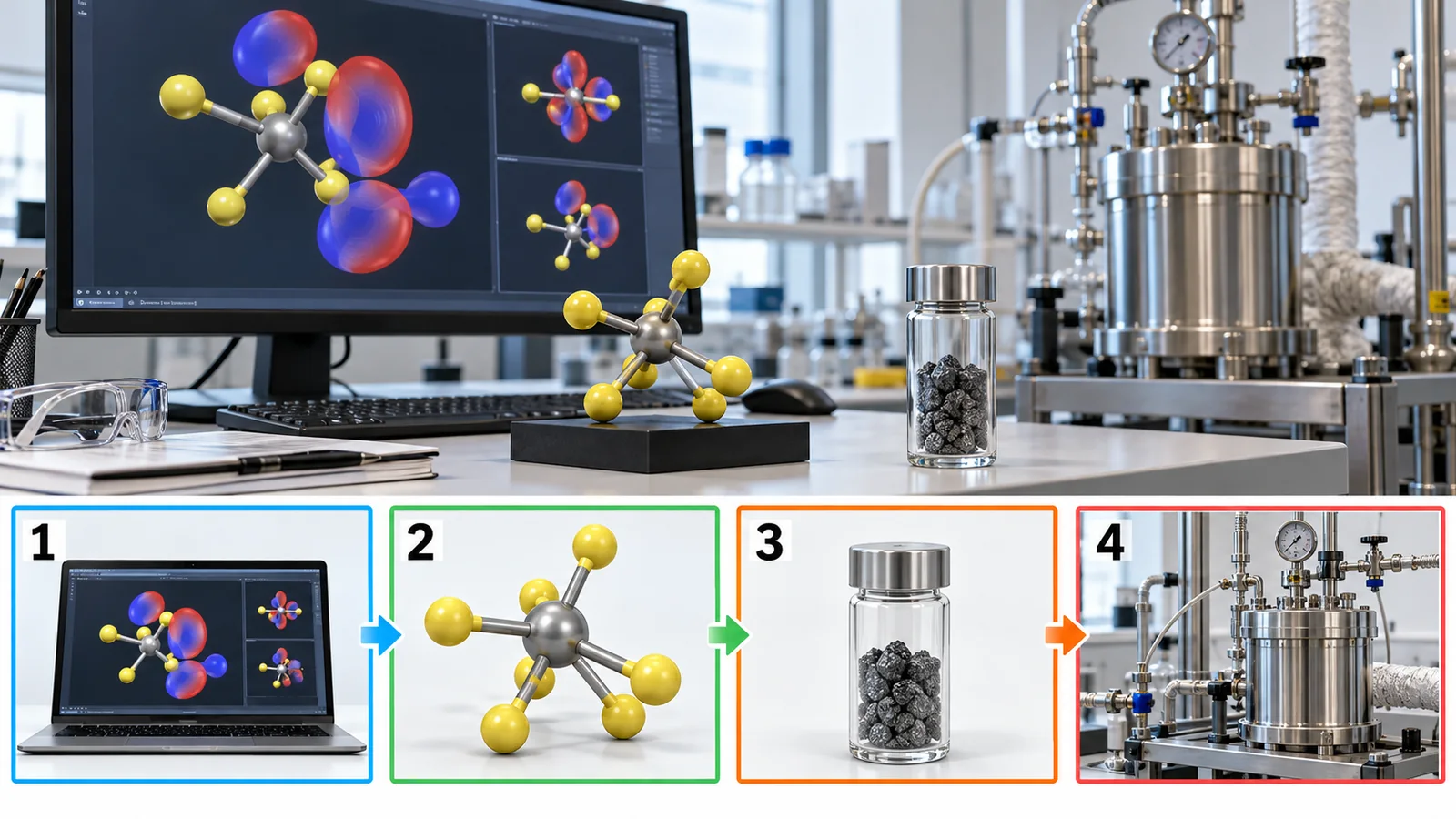
**Fig. 11. Conceptual illustration generated with ImageGen.** A scene linking a material (a catalyst) with molecular simulation. The target of quantum simulation is the electron behaviour of such materials. It does not depict any real facility, product or calculation result. Not an actual product, facility, dimensional specification or measurement. Distinguish enlarged models from full-scale scenes.

A materials engineer's view 1: when and where will a quantum computer help in materials simulation?

The properties of catalysts, battery materials, magnets and superconductors are set by the quantum behaviour of electrons. Quantum simulation is expected to be a way of treating this directly. The assessment, however, is cautious. Lee and colleagues conclude that for ground-state energies evidence for an exponential quantum advantage across chemistry has not yet been found Sourced [Ref. 26]. Resource estimates have been shown for specific targets such as FeMoco, but results on machines stay with small molecules [Refs. 24, 25, 22].

For a materials engineer, telling apart the problems where the best classical methods (such as density-functional theory) are enough from those where they are not (transition-metal catalysts with strong electron correlation, strongly correlated magnets and superconductors) is the entrance to using a quantum computer on materials (our commentary; AI-driven materials discovery is covered in the series' Materials Informatics articles, and quantum chemistry in our article on quantum chemistry and materials simulation).

A materials engineer's view 2: the "count" of an algorithm sets the error rate that is needed

As the "Coherence and Fidelity" article showed, without error correction the success probability falls to about 37% after about 1/ε gates. Apply this to Grover. For a search with N = 10⁹ there are about 24,836 steps; if each step needs, say, 100 gates for the oracle and the reflection, the total is about 2.5 million gates. To succeed without error correction, the error rate per gate would have to be about 4×10⁻⁷ or below Our calculation (1/2.5 million ≈ 4×10⁻⁷; "100 gates" is an illustrative assumption). That is far lower than the reported examples in the earlier article (levels such as 10⁻⁴ to 10⁻³). So practical-scale algorithms presuppose quantum error correction [Refs. 14, 6].

For a materials engineer, error correction means lining up and controlling millions of physical qubits of the same quality. How precisely Josephson-junction frequencies can be matched (frequency crowding), wiring and packaging, the heat load at cryogenic temperatures, and the scatter of material defects directly constrain scaling (our commentary; see Chapter 10 of the gates article, our article on cryogenics and control, and our article on materials and fabrication for quantum computers).

A materials engineer's view 3: the "input" and "output" problem: the cost of turning data into a quantum state

In quantum algorithms for machine learning and linear algebra, the cost of loading large data as a quantum state (input) and of extracting the result (output) can decide the overall speed. Aaronson says that the real speed-up cannot be known without checking such "fine print" Sourced [Ref. 29]. When you read that measurement data on materials (spectra, microscope images) will be analysed on a quantum computer, first check how the data is turned into a quantum state (our commentary).

11. How to read evaluations and standards

The "performance" of a quantum algorithm is read in three layers: complexity (how counts and gate numbers grow), estimates of the resources needed (the number of physical and logical qubits, and time), and results of execution on real machines. Each is measured differently, and there are almost no standards. The table sets out what we could confirm (checked 16 October 2026).

What is measured	Representative benchmark or evaluation method (name, source)	Standards and guidance (NIST, ISO/IEC, IEEE and others)	How to read it
Theoretical speed of an algorithm	Analysis of complexity (query count, gate count). The survey by Montanaro [2]; the survey by Dalzell et al. (overall complexity including error correction) [27]; the Quantum Algorithm Zoo [3] Sourced	Could not be confirmed (there is no standard)	Asymptotic assessments that often leave out constant factors and error-correction overhead [14]
Estimates of the resources needed	Gidney and Ekerå (2021), Gidney (2025), Reiher et al. (2017), Lee et al. (2021) [31, 6, 24, 25] Sourced	Could not be confirmed	Estimates under assumptions (error rate, code, connectivity, time). Not forecasts Not yet confirmed
Execution on machines	Small demonstrations (Vandersypen et al., Kandala et al., Xue et al.) [16, 22, 23]. Classical re-evaluations (Pan et al., Tindall et al.) [33, 35] Sourced	Could not be confirmed	Beware simplifications that depend on knowing the answer [17]. Read company claims side by side with classical re-evaluations
Application-oriented performance	Application-oriented benchmarks (Lubinski et al., 2023) [37] Sourced / DARPA QBI (a program to verify utility scale, with 2033 as its target) [36] Not yet confirmed	Could not be confirmed (IEEE P7131 has a working group on performance metrics, but we found no published standard) [38]	QBI is a national evaluation program, not a standard. A target year is not a guarantee
Effect on cryptography (standards to prepare for Shor)	— (not an evaluation but transition standards and guidance)	NIST FIPS 203 (Module-Lattice-Based Key-Encapsulation Mechanism Standard), FIPS 204 (Module-Lattice-Based Digital Signature Standard) and FIPS 205 (Stateless Hash-Based Digital Signature Standard): all finalised on 13 August 2024 [39, 40, 41] Sourced / NIST IR 8547 (Transition to Post-Quantum Cryptography Standards): initial public draft dated 12 November 2024; we found no final version at the check date [42] Not yet confirmed	We limit ourselves to saying that standards and guidance exist. The time when encryption might be broken cannot be predicted with confidence. Post-quantum cryptography is covered in our articles on post-quantum cryptography and on migration
Terms	— (terminology, not evaluation)	ISO/IEC 4879:2024 "Information technology — Quantum computing — Vocabulary" (edition 1, May 2024, IEC/ISO JTC 3) [43] Sourced / IEEE P7130 "Standard for Quantum Technologies Definitions" (on IEEE's page an active PAR, that is, a project under development; PAR approved 23 September 2021) [44] Not yet confirmed	A vocabulary, not a standard that decides pass or fail for performance. We have not read the texts and state none of their definitions

The arrangement of this table is our own organisation (Our calculation). NIST numbers, titles and dates were checked on NIST CSRC's official pages, the ISO number, title and date on ISO's committee page, and the IEEE status on IEEE SA's pages (checked 16 October 2026). Standard texts are paid or unread, so we limit ourselves to title and scope.

Reading notes (for materials engineers)

Read "faster" together with its kind and conditions: exponential, quadratic or oracle-only? Check the error-correction overhead, the input and output costs, and the comparison with the best classical methods
A resource estimate is not a forecast: if the assumptions (a 0.1% error rate, a 1 µs surface-code cycle and so on) change, the numbers change. We cannot write "encryption will be broken in such-and-such a year"
Read machine demonstrations and company claims side by side with re-evaluations: as classical methods advance, tasks once called "impossible classically" can be solved classically [Refs. 33, 35]
Check whether a standard is a recommendation or a requirement: a NIST FIPS is a federal standard (a standard for cryptographic methods), not a standard for the performance of quantum algorithms. ISO/IEC 4879 is a vocabulary, and IEEE P7130 and P7131 are under development

12. Glossary

Quantum algorithm: A procedure of quantum gates and measurement that solves a problem, designed so that interference boosts the right answer.

Interference: Adding waves. It reinforces waves of the right answer and weakens wrong ones. The core of quantum algorithms.

Amplitude: The number from which a probability is built (a wave height). Positive or negative; it can cancel.

Oracle: A box with unknown contents that counts as one query by convention, such as a box that checks whether a candidate wins.

Query: One use of the oracle. One yardstick for counting an algorithm's speed.

Deutsch's problem: The smallest example: telling whether a function is constant or balanced with one query.

Deutsch–Jozsa: Deutsch's problem with n input bits. The exponential gap holds only against deterministic classical methods.

Grover search: An algorithm that searches without structure in about √N steps. A quadratic speed-up, and optimal.

Amplitude amplification: A method that enlarges the winner's wave by repeated reflection (the generalisation of Grover).

Shor's algorithm: Solves factoring and discrete logarithms in polynomial time, using a quantum Fourier transform to find a period.

Period (order): The length after which the remainder of a^x divided by N repeats. What Shor's algorithm finds.

Quantum Fourier transform: A quantum transform that turns a periodic pattern into frequencies. It extracts the period by interference.

Quantum phase estimation: A component that reads the eigenvalue (the rotation angle) of an operation U using readout qubits and interference.

Eigenstate, eigenvalue: A state whose direction an operation does not change, and the phase (or energy) it picks up.

Hamiltonian: The expression (operator) for the energy of a system.

Quantum simulation: Imitating a quantum system on a quantum computer (Feynman).

Variational method (VQE): A method combining classical optimisation with a quantum circuit to search for the ground-state energy.

HHL: A quantum algorithm for linear equations. Conditions such as input and output need care.

BQP: The class of problems a quantum computer can solve in polynomial time with a small error probability.

NP-complete problem: A representative hard problem of searching many candidates for one that meets conditions.

Resource estimate: An estimate, under assumptions, of the qubits and time needed to run an algorithm.

Post-quantum cryptography (PQC): Cryptography believed to resist quantum computers. NIST has published standards.

Utility: Obtaining meaningful results at a scale beyond brute-force classical computation. Treated as a company claim.

13. References (primary sources)

Cleve R. et al. "Quantum algorithms revisited", Proc. R. Soc. Lond. A 454, 339–354 (1998), DOI 10.1098/rspa.1998.0164 — doi.org/10.1098/rspa.1998.0164
Montanaro A. "Quantum algorithms: an overview", npj Quantum Inf. 2, 15023 (2016), DOI 10.1038/npjqi.2015.23 — doi.org/10.1038/npjqi.2015.23
Jordan S. "Quantum Algorithm Zoo" (catalog of quantum algorithms) (checked 16 October 2026) — quantumalgorithmzoo.org
Bennett C. H., Bernstein E., Brassard G., Vazirani U. "Strengths and Weaknesses of Quantum Computing", SIAM J. Comput. 26, 1510–1523 (1997), DOI 10.1137/S0097539796300933 — doi.org/10.1137/S0097539796300933
Google Quantum AI "Quantum error correction below the surface code threshold", Nature 638, 920–926 (2025), DOI 10.1038/s41586-024-08449-y (arXiv:2408.13687) — doi.org/10.1038/s41586-024-08449-y
Gidney C. "How to factor 2048 bit RSA integers with less than a million noisy qubits", arXiv:2505.15917 (2025) — arxiv.org/abs/2505.15917
Deutsch D. "Quantum theory, the Church–Turing principle and the universal quantum computer", Proc. R. Soc. Lond. A 400, 97–117 (1985), DOI 10.1098/rspa.1985.0070 — doi.org/10.1098/rspa.1985.0070
Deutsch D., Jozsa R. "Rapid solution of problems by quantum computation", Proc. R. Soc. Lond. A 439, 553–558 (1992), DOI 10.1098/rspa.1992.0167 — doi.org/10.1098/rspa.1992.0167
Simon D. R. "On the Power of Quantum Computation", SIAM J. Comput. 26, 1474–1483 (1997), DOI 10.1137/S0097539796298637 — doi.org/10.1137/S0097539796298637
Bernstein E., Vazirani U. "Quantum Complexity Theory", SIAM J. Comput. 26, 1411–1473 (1997), DOI 10.1137/S0097539796300921 — doi.org/10.1137/S0097539796300921
Grover L. K. "A fast quantum mechanical algorithm for database search", Proc. 28th ACM STOC, 212–219 (1996), DOI 10.1145/237814.237866 — doi.org/10.1145/237814.237866
Boyer M. et al. "Tight Bounds on Quantum Searching", Fortschr. Phys. 46, 493–505 (1998), arXiv:quant-ph/9605034 — arxiv.org/abs/quant-ph/9605034
Zalka C. "Grover's quantum searching algorithm is optimal", Phys. Rev. A 60, 2746–2751 (1999), DOI 10.1103/PhysRevA.60.2746 — doi.org/10.1103/PhysRevA.60.2746
Babbush R. et al. "Focus beyond Quadratic Speedups for Error-Corrected Quantum Advantage", PRX Quantum 2, 010103 (2021), DOI 10.1103/PRXQuantum.2.010103 — doi.org/10.1103/PRXQuantum.2.010103
Shor P. W. "Polynomial-Time Algorithms for Prime Factorization and Discrete Logarithms on a Quantum Computer", SIAM J. Comput. 26, 1484–1509 (1997), DOI 10.1137/S0097539795293172 — doi.org/10.1137/S0097539795293172
Vandersypen L. M. K. et al. "Experimental realization of Shor's quantum factoring algorithm using nuclear magnetic resonance", Nature 414, 883–887 (2001), DOI 10.1038/414883a — doi.org/10.1038/414883a
Smolin J. A., Smith G., Vargo A. "Oversimplifying quantum factoring", Nature 499, 163–165 (2013), DOI 10.1038/nature12290 (arXiv:1301.7007 "Pretending to factor large numbers on a quantum computer") — doi.org/10.1038/nature12290
Kitaev A. Yu. "Quantum measurements and the Abelian Stabilizer Problem", arXiv:quant-ph/9511026 (1995) — arxiv.org/abs/quant-ph/9511026
Feynman R. P. "Simulating physics with computers", Int. J. Theor. Phys. 21, 467–488 (1982), DOI 10.1007/BF02650179 — doi.org/10.1007/BF02650179
Lloyd S. "Universal Quantum Simulators", Science 273, 1073–1078 (1996), DOI 10.1126/science.273.5278.1073 — doi.org/10.1126/science.273.5278.1073
Aspuru-Guzik A. et al. "Simulated Quantum Computation of Molecular Energies", Science 309, 1704–1707 (2005), DOI 10.1126/science.1113479 — doi.org/10.1126/science.1113479
Kandala A. et al. "Hardware-efficient variational quantum eigensolver for small molecules and quantum magnets", Nature 549, 242–246 (2017), DOI 10.1038/nature23879 — doi.org/10.1038/nature23879
Xue X. et al. "Quantum logic with spin qubits crossing the surface code threshold", Nature 601, 343–347 (2022), DOI 10.1038/s41586-021-04273-w — doi.org/10.1038/s41586-021-04273-w
Reiher M. et al. "Elucidating reaction mechanisms on quantum computers", Proc. Natl. Acad. Sci. USA 114, 7555–7560 (2017), DOI 10.1073/pnas.1619152114 — doi.org/10.1073/pnas.1619152114
Lee J. et al. "Even More Efficient Quantum Computations of Chemistry Through Tensor Hypercontraction", PRX Quantum 2, 030305 (2021), DOI 10.1103/PRXQuantum.2.030305 — doi.org/10.1103/PRXQuantum.2.030305
Lee S. et al. "Evaluating the evidence for exponential quantum advantage in ground-state quantum chemistry", Nat. Commun. 14, 1952 (2023), DOI 10.1038/s41467-023-37587-6 — doi.org/10.1038/s41467-023-37587-6
Dalzell A. M. et al. "Quantum algorithms: A survey of applications and end-to-end complexities", arXiv:2310.03011 (2023); Cambridge University Press (2025) — arxiv.org/abs/2310.03011
Harrow A. W., Hassidim A., Lloyd S. "Quantum Algorithm for Linear Systems of Equations", Phys. Rev. Lett. 103, 150502 (2009), DOI 10.1103/PhysRevLett.103.150502 — doi.org/10.1103/PhysRevLett.103.150502
Aaronson S. "Read the fine print", Nat. Phys. 11, 291–293 (2015), DOI 10.1038/nphys3272 — doi.org/10.1038/nphys3272
Tang E. "A quantum-inspired classical algorithm for recommendation systems", Proc. 51st ACM STOC, 217–228 (2019), DOI 10.1145/3313276.3316310 — doi.org/10.1145/3313276.3316310
Gidney C., Ekerå M. "How to factor 2048 bit RSA integers in 8 hours using 20 million noisy qubits", Quantum 5, 433 (2021), DOI 10.22331/q-2021-04-15-433 — doi.org/10.22331/q-2021-04-15-433
Arute F. et al. (Google AI Quantum) "Quantum supremacy using a programmable superconducting processor", Nature 574, 505–510 (2019), DOI 10.1038/s41586-019-1666-5 — doi.org/10.1038/s41586-019-1666-5
Pan F., Chen K., Zhang P. "Solving the Sampling Problem of the Sycamore Quantum Circuits", Phys. Rev. Lett. 129, 090502 (2022), DOI 10.1103/PhysRevLett.129.090502 — doi.org/10.1103/PhysRevLett.129.090502
Kim Y. et al. "Evidence for the utility of quantum computing before fault tolerance", Nature 618, 500–505 (2023), DOI 10.1038/s41586-023-06096-3 — doi.org/10.1038/s41586-023-06096-3
Tindall J. et al. "Efficient Tensor Network Simulation of IBM's Eagle Kicked Ising Experiment", PRX Quantum 5, 010308 (2024), DOI 10.1103/PRXQuantum.5.010308 — doi.org/10.1103/PRXQuantum.5.010308
DARPA "Quantum Benchmarking Initiative (QBI)" (checked 16 October 2026) — darpa.mil/research/programs/quantum-benchmarking-initiative
Lubinski T. et al. "Application-Oriented Performance Benchmarks for Quantum Computing", IEEE Trans. Quantum Eng. 4, 1–32 (2023), DOI 10.1109/TQE.2023.3253761 — doi.org/10.1109/TQE.2023.3253761
IEEE SA "Quantum Benchmarking Working Group P7131" (page of the working group on quantum computing performance metrics; checked 16 October 2026) — sagroups.ieee.org/7131
NIST "FIPS 203, Module-Lattice-Based Key-Encapsulation Mechanism Standard" (13 August 2024; checked 16 October 2026) — csrc.nist.gov/pubs/fips/203/final
NIST "FIPS 204, Module-Lattice-Based Digital Signature Standard" (13 August 2024; checked 16 October 2026) — csrc.nist.gov/pubs/fips/204/final
NIST "FIPS 205, Stateless Hash-Based Digital Signature Standard" (13 August 2024; checked 16 October 2026) — csrc.nist.gov/pubs/fips/205/final
NIST "IR 8547, Transition to Post-Quantum Cryptography Standards" (initial public draft) (initial public draft, 12 November 2024; no final version found at the check date) — csrc.nist.gov/pubs/ir/8547/ipd
ISO/IEC "ISO/IEC 4879:2024 Information technology — Quantum computing — Vocabulary" (edition 1, May 2024, IEC/ISO JTC 3; checked on ISO's committee page) — iso.org/standard/80432.html
IEEE SA "IEEE P7130 Draft Standard for Quantum Technologies Definitions" (project page) (active PAR, approved 23 September 2021; checked 16 October 2026) — standards.ieee.org/ieee/7130/10680/

14. Claim-to-source audit

Claim in the text	Basis	Category
The common pattern of quantum algorithms: interference of computational paths enhances correct outcomes and suppresses erroneous ones; many algorithms can be understood as cases of phase estimation	Abstract of Cleve et al. (1998) Reference 1 https://doi.org/10.1098/rspa.1998.0164	Sourced
Surveys organising quantum algorithms by size of speed-up (exponential, quadratic and so on) and by application with technical caveats (including error-correction overhead); a catalog of algorithms and kinds of speed-up	Montanaro (2016), Dalzell et al., the Quantum Algorithm Zoo Reference 2 https://doi.org/10.1038/npjqi.2015.23 Reference 27 https://arxiv.org/abs/2310.03011 Reference 3 https://quantumalgorithmzoo.org	Sourced
That Deutsch's problem needs one quantum query versus two deterministic classical queries at n = 1; that Deutsch–Jozsa is easy probabilistically with O(1) queries and the gap holds only against deterministic classical methods; the Simon and Bernstein–Vazirani problems	Titles and bibliographic data of Deutsch (1985), Deutsch and Jozsa (1992), Simon, Bernstein and Vazirani; the Quantum Algorithm Zoo Reference 7 https://doi.org/10.1098/rspa.1985.0070 Reference 8 https://doi.org/10.1098/rspa.1992.0167 Reference 9 https://doi.org/10.1137/S0097539796298637 Reference 10 https://doi.org/10.1137/S0097539796300921 Reference 3 https://quantumalgorithmzoo.org	Sourced
That Grover search needs O(√N) queries, a quadratic speed-up over classical Ω(N), and is optimal; that for unstructured search NP cannot be solved in quantum time below 2^(n/2) (relative to an oracle)	Titles and abstracts of Grover (1996), Bennett et al., Boyer et al., Zalka; the Quantum Algorithm Zoo Reference 11 https://doi.org/10.1145/237814.237866 Reference 4 https://doi.org/10.1137/S0097539796300933 Reference 12 https://arxiv.org/abs/quant-ph/9605034 Reference 13 https://doi.org/10.1103/PhysRevA.60.2746 Reference 3 https://quantumalgorithmzoo.org	Sourced
The conclusion that quadratic speed-ups will not enable quantum advantage on early fault-tolerant devices because of error-correction constant-factor overhead (quartic speed-ups look more practical)	Abstract of Babbush et al. (2021) Reference 14 https://doi.org/10.1103/PRXQuantum.2.010103	Sourced
That Shor's factoring runs in polynomial time; Õ(n³) versus the classical number field sieve at about 2^Õ(n^(1/3)) (believed)	Title of Shor (1997); the Quantum Algorithm Zoo Reference 15 https://doi.org/10.1137/S0097539795293172 Reference 3 https://quantumalgorithmzoo.org	Sourced
The NMR factoring of N = 15 (seven nuclear spins, 2001); that many small demonstrations relied on simplifications that depended on knowing the factors in advance; that the measure of difficulty is the length of the period found	Abstracts of Vandersypen et al. (2001) and Smolin et al. (2013) Reference 16 https://doi.org/10.1038/414883a Reference 17 https://doi.org/10.1038/nature12290	Sourced
The formulation of quantum phase estimation and its relation to other algorithms	Abstracts of Kitaev (1995) and Cleve et al. (1998) Reference 18 https://arxiv.org/abs/quant-ph/9511026 Reference 1 https://doi.org/10.1098/rspa.1998.0164	Sourced
The idea of quantum simulation (Feynman, Lloyd, Aspuru-Guzik et al.); small machine examples (up to six qubits, up to BeH2; a molecular energy on silicon spins)	Titles and abstracts of the papers Reference 19 https://doi.org/10.1007/BF02650179 Reference 20 https://doi.org/10.1126/science.273.5278.1073 Reference 21 https://doi.org/10.1126/science.1113479 Reference 22 https://doi.org/10.1038/nature23879 Reference 23 https://doi.org/10.1038/s41586-021-04273-w	Sourced
Resource estimates for FeMoco and others (theoretical estimates); the assessment that evidence for an exponential quantum advantage in ground-state chemistry has not yet been found	Abstracts of Reiher et al. (2017) and Lee et al. (2021, 2023) Reference 24 https://doi.org/10.1073/pnas.1619152114 Reference 25 https://doi.org/10.1103/PRXQuantum.2.030305 Reference 26 https://doi.org/10.1038/s41467-023-37587-6	Sourced
The proposal of a superpolynomial speed-up for HHL; that details such as input and output must be checked; that a classical algorithm matched the speed for the recommendation-system problem	Title of Harrow et al. (2009), Aaronson (2015), Tang (2019) Reference 28 https://doi.org/10.1103/PhysRevLett.103.150502 Reference 29 https://doi.org/10.1038/nphys3272 Reference 30 https://doi.org/10.1145/3313276.3316310	Sourced
Resource estimates for RSA-2048: 20 million qubits and 8 hours (2019, 2021); under a million qubits and under a week (2025). Assumptions: a square grid, an error rate of 0.1%, a 1 µs surface-code cycle, a 10 µs reaction time	Abstracts of Gidney and Ekerå (2021) and Gidney (2025) Reference 31 https://doi.org/10.22331/q-2021-04-15-433 Reference 6 https://arxiv.org/abs/2505.15917	Sourced
The error-correction experiment: a distance-7 surface code with 101 qubits (company report)	Abstract of Google Quantum AI (2024, 2025) Reference 5 https://doi.org/10.1038/s41586-024-08449-y	Sourced
The company claim for random-circuit sampling (about 200 s versus an estimated 10,000 years) and the classical re-evaluation (512 GPUs, about 15 hours); the utility claim and the tensor-network classical simulation	Abstracts of Arute et al. (2019), Pan et al. (2022), Kim et al. (2023), Tindall et al. (2024) Reference 32 https://doi.org/10.1038/s41586-019-1666-5 Reference 33 https://doi.org/10.1103/PhysRevLett.129.090502 Reference 34 https://doi.org/10.1038/s41586-023-06096-3 Reference 35 https://doi.org/10.1103/PRXQuantum.5.010308	Sourced
That DARPA's QBI is a program to test whether an industrially useful quantum computer is possible by 2033 (a target of a national evaluation program)	DARPA's official page (checked 16 October 2026) Reference 36 https://www.darpa.mil/research/programs/quantum-benchmarking-initiative	Not yet confirmed
The proposal of application-oriented benchmarks; that the IEEE P7131 working group is active and we found no published standard	Title of Lubinski et al. (2023); IEEE SA page Reference 37 https://doi.org/10.1109/TQE.2023.3253761 Reference 38 https://sagroups.ieee.org/7131	Not yet confirmed
That NIST FIPS 203, 204 and 205 were finalised on 13 August 2024 (titles); that the initial public draft of NIST IR 8547 is dated 12 November 2024 (no final version found)	NIST CSRC official pages Reference 39 https://csrc.nist.gov/pubs/fips/203/final Reference 40 https://csrc.nist.gov/pubs/fips/204/final Reference 41 https://csrc.nist.gov/pubs/fips/205/final Reference 42 https://csrc.nist.gov/pubs/ir/8547/ipd	Sourced
The number, title and date of ISO/IEC 4879:2024 "Information technology — Quantum computing — Vocabulary" (edition 1, May 2024, IEC/ISO JTC 3); that IEEE P7130 is under development (active PAR, approved 23 September 2021)	ISO's committee page, IEEE SA page Reference 43 https://www.iso.org/standard/80432.html Reference 44 https://standards.ieee.org/ieee/7130/10680/	Sourced
The Deutsch amplitude table (four functions), the classical randomized error (n = 20, 10 queries, about 0.195%), Grover amplitudes and probabilities (N = 8), the optimal-count table, the period for N = 15, the peaks of the 64-point and 128-point Fourier transforms, the phase-estimation distribution (φ = 1/3, 4 bits), the Grover step and error-rate estimate (about 2.5 million gates, about 4×10⁻⁷), the ratios (9,900 and 198,000)	Our own calculation (Python, NumPy). Not the results of any real device. The "100 gates" per step is an illustrative assumption	Our calculation
Primary sources on machine demonstrations of Deutsch or Grover, the text of ISO/IEC 4879, the publication state of IEEE P7131 and a final NIST IR 8547 could not be confirmed from the primary sources available in this survey, so they are not stated	Not confirmed within the scope of this survey	commentary
Readings such as "parallel computation makes it fast is inaccurate", "Deutsch–Jozsa gaps hold only against deterministic classical methods", "Grover does not make web search instant", "quantum does not solve all NP-complete problems quickly is wrong", and the analogies with their limits	Our own organisation and commentary based on the published material; not views expressed by the organisations cited	commentary
That Figs. 1 to 11 are explanatory drawings and not observations of real data, and that Figs. 1 and 11 are ImageGen-generated conceptual illustrations	Note in this article	commentary

Last updated: 16 October 2026. Sources are limited to primary material (surveys, peer-reviewed papers, arXiv papers, the Quantum Algorithm Zoo, and official NIST, DARPA, ISO and IEEE pages). Company claims are treated as company claims, and where a classical re-evaluation exists we show both. The numerical examples (amplitudes, probabilities, counts, periods, the phase-estimation distribution, the error-rate estimate) are our own illustrative calculations, not results from real devices. The resource estimates are theory under assumptions, not forecasts. We give no procedure for, and no timing of, breaking encryption. We could not confirm some primary sources on machine demonstrations, the text of the standards, the publication state of IEEE P7131 or a final NIST IR 8547, so we do not state them. All figures are explanatory conceptual diagrams or drawings that include our own calculations; Figs. 1 and 11 are ImageGen-generated conceptual illustrations.

Illustration update: 17 October 2026. References to vector drawings in the article and source tables describe the retained original SVGs. See each current caption for the foreground image format and reading guide. ImageGen illustrations are not measurements or photographs of actual products; original SVGs, values and sources remain available in expandable references.