TECHNOLOGY EXPLAINER
Superconducting Qubits
― How an electrical circuit becomes a qubit, and the materials behind it
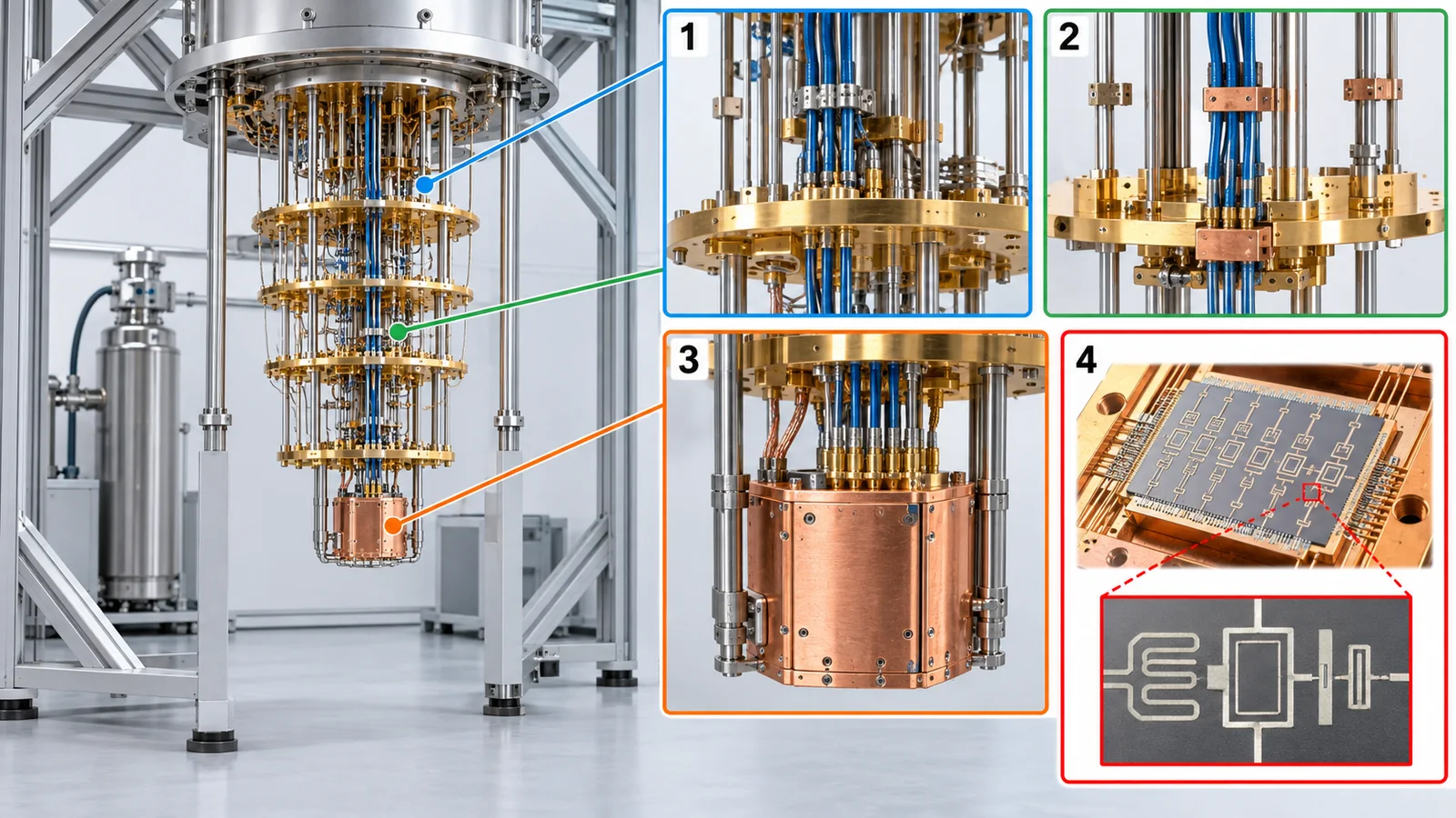
A superconducting qubit is a superconducting electrical circuit drawn on a chip and cooled to very low temperature so that it behaves like an "artificial atom." An ordinary circuit cannot be a qubit as it is. Only after a part called a Josephson junction is added does it become a circuit in which just "0 and 1" can be controlled. This article explains, step by step and with figures and small numerical examples: (1) why a circuit can be a qubit, (2) how it is controlled and read out, (3) what its strengths and weaknesses are, and (4) which materials and manufacturing steps support it. The later chapters summarize the state of play as of the check date (16 October 2026), keeping achievements and plans apart.
- In three lines / what to know first / where this sits in the series
- Recap: a qubit is an "arrow"
- Why can a circuit be a qubit? (1) The evenly spaced ladder
- Why can a circuit be a qubit? (2) The Josephson junction and the transmon
- Why cool it to such a low temperature?
- Control and readout
- The key points on a common "card," and a side-by-side with the other three approaches
- Materials and manufacturing: what decides the lifetime
- Where things stand (checked 16 October 2026) and plans
- Limits, what we could not confirm, and a summary
- How to read evaluations and standards
- Glossary
- References (primary sources)
- Claim-to-source audit
Sourced = stated in a published source (with a link)
Our calculation = a value this article computed from stated assumptions
Not yet confirmed = plans, targets, drafts and other items that are not settled
Readings for materials research and analogies are marked as commentary. An inference is shown in bold.
A quantum-computing number means little unless it comes with what was measured and how. Here, error rates, fidelities and lifetimes come with the approach, the thing measured, whether it is an average or a best value, and the date. Company announcements are labeled as the company's claims, and plans and targets are shown as Not yet confirmed, kept apart from achieved facts. The temperature and size examples in Chapters 4 and 5 are our own "feel-for-the-size" calculations, not the performance of any real machine. We did not read the full texts of the standards (ISO/IEC, IEEE), which are paid; we give only titles and status. We do not tell lies to keep things simple. Every analogy comes with its limits.
1. In three lines / what to know first / where this sits in the series
- A superconducting qubit is a small electrical circuit made of superconductors (about 1 mm across) whose "lowest two energy steps" are used as 0 and 1. Because it is drawn on a chip, it is also called an "artificial atom"[Ref. 1]Sourced
- An ordinary circuit cannot be a qubit as it is. Its energy steps are evenly spaced, so we cannot aim at "just 0 and 1." Adding a Josephson junction makes the gaps uneven, so a microwave can move just the two chosen steps[Ref. 1, 2]Sourced
- Control uses microwave pulses; readout uses a small shift in a resonator's response. It must run at a very low temperature, about 20 mK. It is fast, but qubit lifetimes are relatively short, and wiring, cooling and fabrication variation are the challenges. Lifetime changes a lot with the materials (tantalum, aluminum, substrate, oxide layers)[Ref. 1, 3]Sourced
A superconducting qubit is "an electrical circuit built so that its energy steps are uneven." The part that makes it so is the Josephson junction, and what decides its performance (lifetime) is the materials: thin films, oxide layers and the substrate.
Prerequisites: none. The arrow picture is recapped in the next chapter (no quantum-mechanics formulas are used).
Place in the series: read this after "The Basics of Quantum Computing" and "Quantum Gates and Circuits." It is easiest to read side by side with the other three approaches (trapped ions, neutral atoms, photonic quantum computers). How lifetimes and error rates are measured is covered in our explainer on coherence and fidelity; refrigerators and wiring in our explainer on cryogenics and control; materials in general in our explainer on materials and manufacturing for quantum computers; and error correction in our explainer on quantum error correction and the surface code.
2. Recap: a qubit is an "arrow"
In this series, a qubit's state is drawn as an arrow from the center of a sphere to its surface. Pointing at the north pole means "0," pointing at the south pole means "1," and pointing in between is a superposition. When the arrow is tilted, a measurement always gives 0 or 1, and the chance of each is set by the tilt. After the measurement the arrow is fixed at a pole, and the old tilt does not come back.
That is wrong. A tilted arrow is not "holding both 0 and 1" but "pointing in a definite direction between 0 and 1." Measure it and you get just one of 0 or 1. A quantum computer's power comes from combining these arrow directions like waves so that the right answer reinforces itself (see our explainer on quantum algorithms).
3. Why can a circuit be a qubit? (1) The evenly spaced ladder
(1) A familiar example: a swing
A swing takes about the same time for one back-and-forth trip whether you swing it a little or a lot. If you push in rhythm, the swing grows larger and larger. The same thing happens in an electrical circuit. Connect a coil (L) and a capacitor (C), and the electricity sloshes back and forth. This is an LC resonator, a relative of the tuning circuit in a radio. In a tiny system such as an atom or a circuit, the energy of this oscillation comes in "discrete steps." Like a staircase, you can only be on step 1, step 2, step 3, and so on. The steps of an LC resonator are all equally spaced (an evenly spaced ladder)[Ref. 1]Sourced.
(2) The problem: with even spacing we cannot use "just 0 and 1"
A qubit needs just two steps, 0 and 1. In an evenly spaced ladder, though, the gaps 0→1, 1→2 and 2→3 all correspond to the same frequency. A microwave at that frequency moves not only 0→1 but also 1→2 and 2→3, so we cannot aim at "just 0 and 1"[Ref. 1].
(3) The fix: make the spacing uneven
When a Josephson junction (next chapter) is added, the circuit stops acting like a plain coil, and the steps become unevenly spaced. If the 1→2 gap is a little smaller than the 0→1 gap, a microwave at the 0→1 frequency moves only 0 and 1, and 1→2 does not respond. The real difference is about 100–300 MHz when the qubit frequency is 3–6 GHz (a few percent)[Ref. 1]Sourced. Even a tiny difference works, because a frequency can be tuned very precisely.
An electron inside an atom cannot sit at any height it likes; it can only sit on "steps" of fixed heights (energies). These are called energy levels. A superconducting circuit, cooled hard and considered only for small oscillations, also has "discrete steps" like an atom. That is why a circuit on a chip is called an "artificial atom." Limits of the analogy: a swing is the motion of a visible object, whereas in a circuit what oscillates is "the amount of electric charge and magnetic flux." A swing can have any energy, but a quantum circuit can only have "discrete steps" — that is where the swing analogy breaks down.
4. Why can a circuit be a qubit? (2) The Josephson junction and the transmon
(1) What is a Josephson junction?
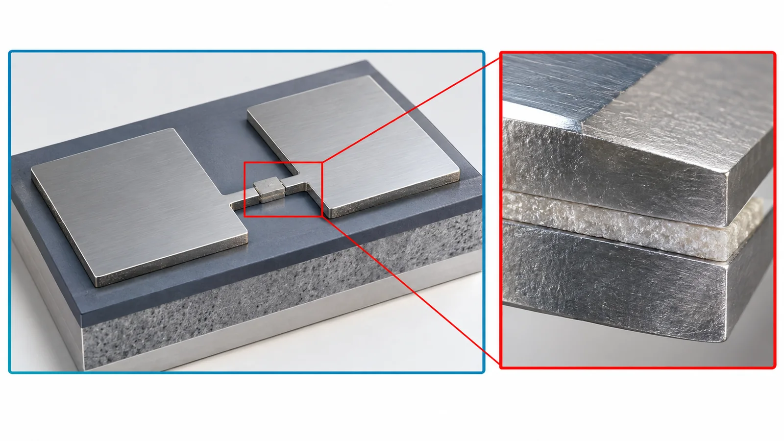
Superconductivity is the state in which a metal, when cooled, has zero electrical resistance so current flows without loss. A Josephson junction is a part in which a very thin non-conducting layer is sandwiched between two superconductors[Ref. 4]Sourced. Pairs of superconducting electrons pass through the thin layer by the tunnel effect (a quantum phenomenon of slipping through a wall). Commentary: the junction acts like "a coil without resistance," but unlike an ordinary coil, its behavior changes as the current grows (it is nonlinear), and that is the crux. The review by Krantz et al. explains that the Josephson junction is the key ingredient that makes the oscillator anharmonic and so lets us pick out a uniquely addressable pair of levels[Ref. 1]Sourced.
(2) The transmon: the form used most today
A circuit in which the junction is wired in parallel with a large capacitor is a transmon, proposed by Koch et al. in 2007[Ref. 2]Sourced. A large capacitor makes the circuit insensitive to fluctuations of nearby charge (noise). In exchange, the size of the unevenness shrinks a little, but enough remains to be useful. Koch et al. showed that when the ratio of the junction's energy to the capacitor's energy (EJ/EC) is made large, the sensitivity to charge noise falls exponentially, while the loss of unevenness falls only as a gentle power law[Ref. 2]Sourced. Real transmons are designed with EJ/EC of 50 or more[Ref. 1]Sourced.
View original SVG, values and sources
Original SVG reference: Drawing that includes our own calculation (vector drawing). Concept diagrams of the junction's cross-section, the circuit, and a chip's appearance. The size ratio (about 1/6,000) in the lower panel is our calculation from "about 1 mm" (Krantz et al. [Ref. 1]) and "about 0.03 μm²" (Place et al. [Ref. 5]).
No. A transmon is a circuit that people designed and built. Unlike a natural atom, its step heights (frequencies) are set by design, but the weakness is that every one comes out a little different (Chapter 8). It is also not tiny like an atom; at about 1 mm it is visible without a microscope[Ref. 1]. The 2025 Nobel Prize in Physics honored experiments (1984–85) that showed quantum tunnelling and energy steps in an electrical circuit large enough to hold in the hand[Ref. 4]Sourced.
5. Why cool it to such a low temperature?
Superconducting qubits are operated at about 20 mK (millikelvin; 0.02 degrees above absolute zero)[Ref. 1]Sourced. It is easy to think "we cool it to make it superconducting," but that alone does not explain it. For example, tantalum becomes superconducting at 4.2 K[Ref. 3]Sourced. We cool it more than two orders of magnitude below that so that heat does not move the qubit by itself.
The energy difference between 0 and 1 is that of one 5 GHz microwave photon (hf). Unless the surrounding thermal energy (kT) is well below this, heat randomly excites the qubit to "1." So we compute the ratio hf/kT (Our calculation). At 20 mK, hf/kT = 12.0, and the chance of being in the heat-excited state is about 6×10⁻⁶. At 100 mK, hf/kT = 2.4 and the chance is about 8%; at 1 K it is about 44%, almost half and half. At room temperature (300 K), hf/kT = 0.0008 and the excited-state probability is about 50%, so 0 and 1 cannot be told apart at all. The average number of "thermal photons" at 5 GHz is about 6×10⁻⁶ at 20 mK and about 1,250 at 300 K.
A dilution refrigerator cools in many stages from room temperature to about 20 mK. In one example, the cooling power of the bottom stage is only 19 μW (0.019 mW) at 20 mK[Ref. 6]Sourced. So the heat flowing in through the wires to the chip and the heat of the control signals together must not exceed a few tens of μW. This becomes a big wall when qubits are scaled to thousands or tens of thousands (see our explainer on cryogenics and control).
This is only half right. To merely make it superconducting, a few kelvin would do (4.2 K for tantalum)[Ref. 3]. We cool it orders of magnitude further to make the thermal energy far smaller than the gap between 0 and 1 (one 5 GHz microwave photon). Thermal noise entering through wires and amplifiers is another problem; in one study, attenuators totaling about 60 dB were put in the drive lines so that the number of thermal-noise photons reaching the bottom stage stays around 10⁻³[Ref. 6]Sourced.
Because the chip's cooling power is so small, the cables that carry signals from room temperature to the cold stages must be materials that conduct electricity but not heat. In the measurements of Krinner et al., stainless-steel and niobium-titanium (NbTi) coaxial cables were chosen as the cables with small passive heat inflow[Ref. 6]Sourced. In general, metals that conduct electricity well also conduct heat well (commentary), so here the challenge is how to resolve the conflicting demands of electricity and heat with materials.
6. Control and readout
(1) One-qubit control: turning the arrow
A microwave pulse tuned to the qubit's frequency turns the arrow. The pulse's length and strength set the angle. For example, a half-strength pulse (π/2 pulse) turns it from the north pole to the equator, and a full-strength pulse (π pulse) turns it from north pole to south pole (see the figure). Rotations about the Z axis can be done just by shifting the phase of the following pulses (a "virtual Z gate"). There is also a trick of shaping the pulse to suppress leakage to unwanted levels (DRAG)[Ref. 1]Sourced.
(2) Two-qubit control: connecting for a moment
When there are two or more qubits, a coupling is made between two of them so they interact for a moment. The review by Krantz et al. describes a CPHASE gate that shifts frequencies to bring two states close (an example by Barends et al.: 43 ns, fidelity 0.9944) and a cross-resonance gate that drives one qubit at the other's frequency (an example shifting a phase by π in about 200 ns)[Ref. 1]Sourced. IBM's current processors (Heron) combine fixed-frequency qubits with couplers whose connection can be tuned on and off (tunable couplers)[Ref. 7]Sourced.
(3) Readout: listening to a resonator's "pitch"
Next to the qubit sits another resonator, the readout resonator. The qubit and the resonator are weakly coupled, and the resonator's resonance frequency (its pitch) shifts slightly depending on whether the qubit is 0 or 1 (dispersive readout). So we send microwaves to the resonator and look at the strength or phase of the returned signal to tell 0 from 1[Ref. 8, 1]Sourced. An experiment that strongly couples a qubit to a resonator at the level of single microwave photons was reported by Wallraff et al. in 2004 (circuit quantum electrodynamics)[Ref. 9]Sourced. The returned signal is extremely faint, so "quantum-limited amplifiers," which add only the minimum noise quantum mechanics allows, are used[Ref. 7]Sourced.
There are two basic times that describe a qubit's quality. T1 is a measure of how long it takes the arrow to tumble from the south pole (1) to the north pole (0), losing energy. T2 is a measure of how long it takes the arrow's "direction (phase)" to lose its alignment. For example, with T1 = 100 μs, the chance that a qubit placed in 1 is still in 1 after 100 μs is about 37% (e⁻¹), and after 200 μs about 14% (Our calculation, assuming exponential decay). How they are measured and defined (T2* versus echo T2, and so on) is explained in our explainer on coherence and fidelity.
7. The key points on a common "card," and a side-by-side with the other three approaches
Here is everything so far as a "card" that answers the series' five shared questions (what it is made of, what 0 and 1 are, how it is controlled, how it is read, strengths and weaknesses). The other three articles use the same card.
Reading the four approaches in the same format
| Item | Superconducting | Trapped ion | Neutral atom | Photonic |
|---|---|---|---|---|
| What the qubit is | A superconducting circuit (e.g., a transmon): an "artificial atom" about 1 mm across, drawn on a chip[Ref. 1] | One atomic ion floated in vacuum by radio-frequency electric fields (e.g., Ba⁺, Yb⁺)[Ref. 11, 12] | One neutral atom caught in vacuum by an optical tweezer, a tightly focused laser beam (e.g., Rb, Cs, Yb)[Ref. 13, 14, 15] | A photon (a particle of light) travelling in a waveguide, a path for light, or in an optical fiber[Ref. 16, 17] |
| How 0 and 1 are told apart | The lowest two energy steps of the circuit[Ref. 1] | Two internal states of the atom (e.g., two hyperfine levels of Ba⁺)[Ref. 12] | Two internal states of the atom (e.g., two hyperfine levels of Rb)[Ref. 13] | Which of two paths the photon takes (e.g., one of two waveguides); it can also be an early or late time slot[Ref. 16, 18] |
| How it is controlled | Microwave pulses. Two-qubit gates use a coupler or the cross-resonance effect[Ref. 1, 7] | Laser light (or microwaves or electrical signals). Two-qubit gates use the shared motion of the ions as a go-between[Ref. 11, 19, 20] | Laser light. In a two-qubit gate, atoms are lifted to a highly excited Rydberg state so that nearby atoms affect each other[Ref. 21, 13] | Interference in an optical circuit and photon detection (measurement). Photons pass through each other, so measurement creates the interaction[Ref. 18, 22] |
| How it is read out | Measure a small shift in the microwave response of a resonator (dispersive readout)[Ref. 8, 9] | Shine light and see whether it fluoresces (bright / dark)[Ref. 11] | Image the fluorescence and see which atoms are bright or dark[Ref. 23] | Photodetectors count which path the photon arrived on (one example runs superconducting nanowire detectors at about 2 K)[Ref. 16] |
| Operating environment | About 20 mK in a dilution refrigerator[Ref. 1] | Ultra-high vacuum. Traps exist at room temperature and in cooled form[Ref. 24, 25] | Lasers and optics around an ultra-high-vacuum chamber. Atoms at about 10 μK, apparatus at room temperature[Ref. 13, 23] | Most circuit parts run at room temperature. Detectors are often cooled[Ref. 17, 16] |
| Example two-qubit gate time | 43 ns (an example by Barends et al.) or about 200 ns (a cross-resonance example)[Ref. 1] | About 70 μs (an example from Helios). One study scanned 3.8 μs to 520 μs[Ref. 12, 24] | Gate pulses are on the order of hundreds of ns (one calibration value in Evered et al.: 275 ns). Rearranging and imaging take longer[Ref. 13, 26] | We could not confirm a representative value |
| Example of two-qubit quality (definitions differ) | EPLG 3.7×10⁻³ as shown on IBM's official page (measurement conditions could not be confirmed)[Ref. 7, 27] | Average infidelity 7.9×10⁻⁴ (Helios, average over all zones of a 98-qubit machine)[Ref. 12] | Fidelity 99.5% (up to 60 atoms in parallel, Evered et al.)[Ref. 13] | "Fusion" fidelity 99.22% (only when detection succeeds; loss not included)[Ref. 16] |
| Strengths | Fast. Semiconductor-style microfabrication can be used[Ref. 1] | Ions of one species are all identical. Control precision is high[Ref. 11, 12] | Many identical atoms can be lined up (6,100). The layout can be changed[Ref. 23, 28] | Easy to link with optical fiber. Optical circuits can be built in a semiconductor factory (the plan)[Ref. 16, 17] |
| Weaknesses | Qubit lifetimes are relatively short. Wiring and cooling; fabrication variation[Ref. 10, 3, 6, 29] | Gates are slow. Scaling adds electrodes, lasers and wiring[Ref. 12, 11] | Atoms get lost. Cycles are slow[Ref. 30, 26] | Photon loss is the biggest challenge. Photons barely interact with each other[Ref. 17, 18] |
The arrangement is commentary; the numbers and facts in each cell come from the references (checked 16 October 2026). The numbers are different quantities under different conditions, so please do not rank the approaches by them.
The answer is "not settled yet." Each has different strengths: speed (superconducting), precision and all-to-all connectivity (ions), large numbers and freedom of layout (neutral atoms), and compatibility with communication (photons). All of them attack the same hard problem — keeping quality while adding qubits — by different routes. The numbers in this article's table have different definitions and conditions, so please do not compare them directly.
8. Materials and manufacturing: what decides the lifetime
(1) Lifetimes are far shorter than the materials' "ideal values"
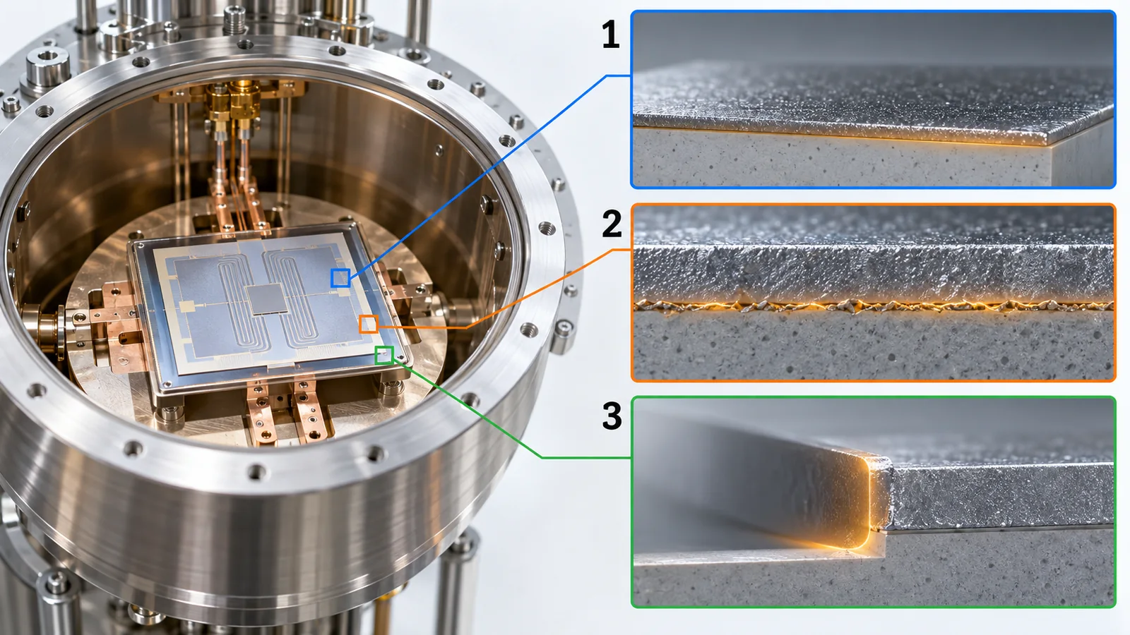
Place et al. point out that because the dielectric loss of high-purity sapphire (the fraction of microwave energy turned into heat) is below 10⁻⁹, T1 could ideally exceed 30 ms, yet the lifetimes of real two-dimensional transmons are much shorter[Ref. 5]Sourced. The gap is thought to come from defects at surfaces and interfaces, and contaminants. The review by Müller et al. explains that circuits made of aluminum or niobium are fundamentally limited by loss from two-level-system (TLS) defects in the surrounding amorphous oxide layers[Ref. 31]Sourced. A TLS is a tiny defect whose energy can take only two values; it soaks up energy from the qubit.
View original SVG, values and sources
Original SVG reference: Concept diagram (vector drawing). A concept diagram of a chip cross-section and candidate places of loss (not to scale). The native oxide on Ta being about 2 nm, and the breakdown of substrate, interface and junction loss, come from Place et al. [Ref. 5] and Bland et al. [Ref. 3].
(2) From niobium to tantalum, from sapphire to silicon
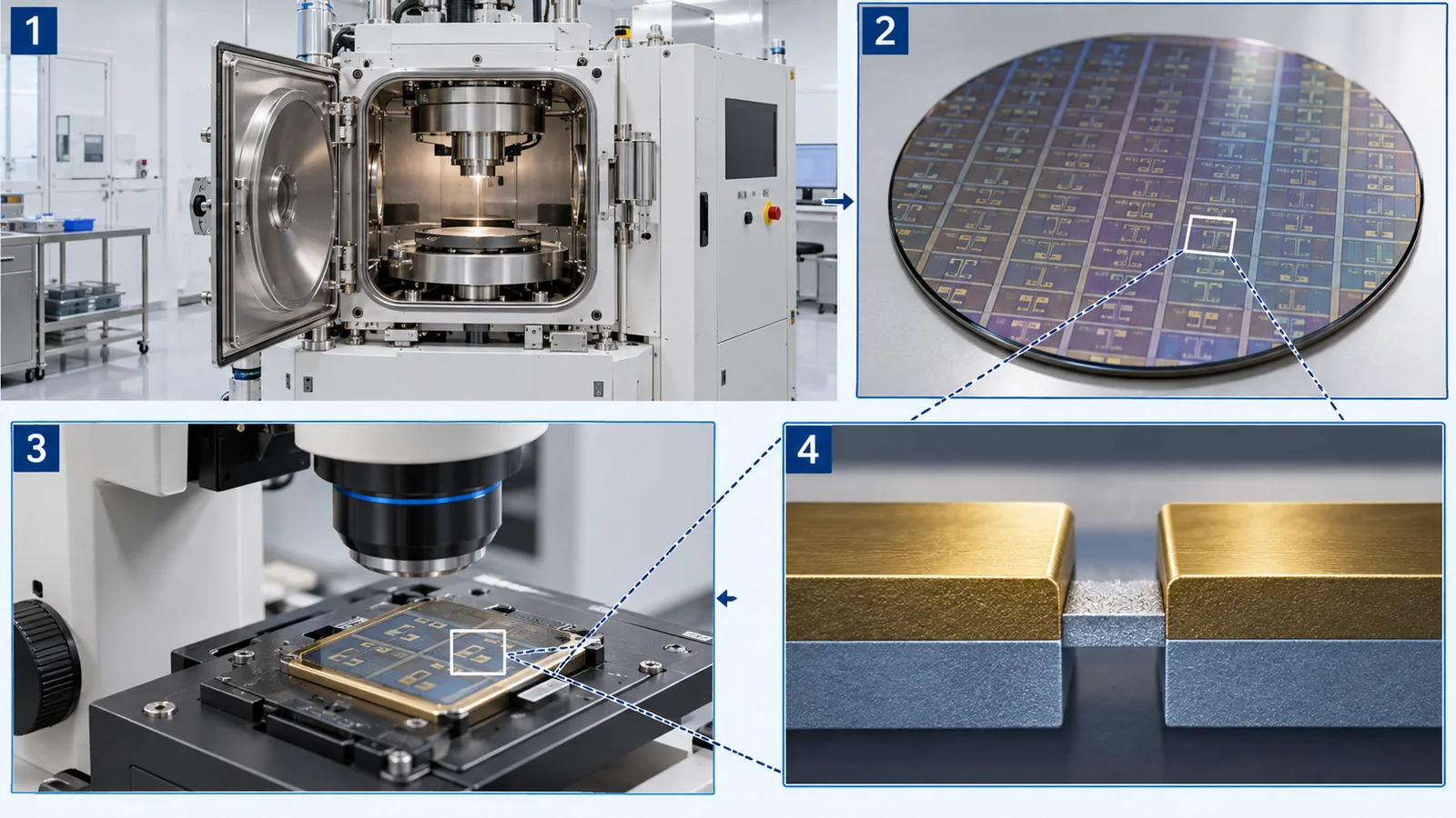
Place et al. replaced the widely used niobium with tantalum for the superconductor of the transmon's capacitor and resonator, and obtained devices whose lifetime and whose phase-retention time (with pulses that cancel phase disturbances) both exceeded 0.3 ms. They confirmed the improved lifetime in 17 devices[Ref. 5]Sourced. They sputtered tantalum (ejecting metal onto the surface) onto a sapphire substrate heated to about 500 °C, shaped it by photolithography and wet etching, and formed the junction from aluminum and its oxide by electron-beam lithography and evaporation. The native oxide on tantalum (Ta₂O₅) is about 2 nm thick[Ref. 5]Sourced. The authors hypothesize that the complicated oxides on niobium create extra loss and that tantalum's oxide reduces it (a hypothesis). Wang et al. compared tantalum, niobium and aluminum films with the same design and the same junction process, and reported tantalum best, aluminum next, niobium last (best T1 of 503 μs)[Ref. 32]Sourced.Bland et al. then replaced the sapphire substrate with high-resistivity silicon, which greatly reduced the loss of the substrate itself, and reported T1 up to 1.68 ms (a maximum quality factor Q of 2.5×10⁷). The tantalum film was grown at 600–650 °C, its superconducting transition temperature was 4.2 K, and no oxide layer was seen at the tantalum–silicon interface. With the loss lowered, decoherence due to the junction became visible, and with low-contamination junction deposition they obtained devices whose phase-retention time (Hahn-echo method) exceeded T1[Ref. 3]Sourced.
Bland et al. summarize that in tantalum-on-sapphire devices the loss comes about equally from surface and bulk dielectrics, and unless both are reduced there is no large improvement[Ref. 3]Sourced. Switching the substrate to silicon lowered the substrate loss, and on that silicon the contribution of the amorphous silicon-oxide layer was estimated to be under 10% of the total surface loss[Ref. 3]Sourced. So the starting point of materials development is separating which layer produces the loss, for example with resonator measurements. Deposition conditions (at higher background pressure a little β-phase tantalum or tantalum silicide forms), cleaning, and oxide control translate directly into qubit lifetime.
(3) Fabrication variation: a small difference in the junction becomes a difference in frequency
A qubit's frequency is set by the junction's properties. In IBM's study, lining up many fixed-frequency transmons required tuning their relative frequencies precisely, which was a difficult step in scaling. Zhang et al. showed a way to heat junctions locally with laser light (laser annealing) and tune frequencies afterwards. Statistics over hundreds of qubits gave a tuning precision of 18.5 MHz, no measurable effect on lifetime, and a median two-qubit gate fidelity of 98.7% on a 65-qubit processor. The authors state that the precision of the junction resistance expressed as frequency (4.7 MHz) is enough for high-yield scaling beyond the 1,000-qubit level (from the abstract of the arXiv version)[Ref. 29]Sourced. In Google's study, because TLS frequencies change with time, the team forecast the TLS frequencies' motion from past lifetime data and set qubit frequencies to avoid them[Ref. 10]Sourced.
As computed in Chapter 4, each side of the junction is about 0.17 μm (an overlap area of 0.03 μm² treated as a square)[Ref. 5]Our calculation. The oxide thickness (a few atomic layers), area and cleanliness of this tiny region connect directly to the qubit's frequency and lifetime. The difficulty resembles that of a semiconductor gate oxide, but qubits add a different strict demand: keeping the frequency within a set band. Inference: being able to measure process reproducibility (within a wafer, wafer to wafer, lot to lot) against a real yardstick — the spread of frequencies in MHz — makes this a field where a materials engineer can readily find process-control metrics.
9. Where things stand (checked 16 October 2026) and plans
(1) Google's error-correction experiment (a peer-reviewed paper by a company research team)
Google Quantum AI used a 105-qubit processor with the surface code, an error-correcting code, and showed that each time the code size (distance) goes up by two, the logical error rate falls by about a factor of 2.14 (Λ = 2.14 ± 0.02). The logical error rate of the distance-7 code (using 101 qubits) is 0.143% ± 0.003% per error-correction cycle, and a cycle takes 1.1 μs. This logical-qubit memory outlived the best physical qubit by a factor of 2.4 (it went beyond break-even). The processor's qubits are reported to have a mean T1 of 68 μs[Ref. 10]Sourced.How to read it: this experiment stores a logical qubit's information (a memory). It does not mean logical operations were run to do useful computation. It is also an experiment by a company's research team; the paper is peer-reviewed (Nature), but we have not confirmed a reproduction of the same experiment by another laboratory (could not confirm).
(2) IBM (statements on the company's official pages)
According to IBM's official page (checked 16 October 2026), the processors currently offered are Heron r1 (133 qubits), Heron r2 and r3 (156 qubits, both with tunable couplers), and Nighthawk (120 qubits on a square lattice, each qubit coupled to four others). The page shows the "quality (EPLG)" of Heron and Nighthawk as 3.7×10⁻³ and says Nighthawk r2 is 25 times faster (values shown by the company; we could not confirm the measurement conditions)[Ref. 7]Sourced.
(3) Japan: Fujitsu and RIKEN
On 22 April 2025, Fujitsu and RIKEN announced a 256-qubit superconducting quantum computer (four times the 64-qubit machine of 2023)[Ref. 33]Sourced. The same announcement said a 1,000-qubit machine is scheduled to be installed in a new building at Fujitsu's site in 2026[Ref. 33]Not yet confirmed. As of the check date we could not confirm an official announcement that the 1,000-qubit machine was completed.
(4) Plans (not yet confirmed): IBM's roadmap
IBM's official roadmap states at the outset that it "represents IBM's current intent" and consists of goals that may change or be withdrawn[Ref. 34]Not yet confirmed. 2026: run circuits of 7,500 gates on up to three 120-qubit Nighthawk modules; prototype an error-correction decoder and demonstrate a single Kookaburra module that combines a logical processing unit with a quantum memory. 2028: 15,000 gates on up to 1,080 qubits. 2029: Starling ("200 qubits," 100 million gates). 2033 and after: Blue Jay ("2000 qubits," 1 billion gates). The page says only "qubits," so whether they are physical or logical qubits cannot be told from the page's text (could not confirm).
This is wrong. IBM's current machines have 120–156 qubits, but the official page gives separate indicators of "quality"[Ref. 7]. What Google's experiment showed is not the qubit count itself but that if the physical error is below the threshold, the logical error rate falls exponentially as more qubits are added (the code is made larger)[Ref. 10]Sourced. Look at qubits as a whole: number and quality (error rate), connectivity, and speed. And "how many qubits" means something entirely different depending on whether they are physical qubits or error-corrected logical qubits. One logical qubit uses many physical qubits (101 qubits in Google's distance-7 code).
10. Limits, what we could not confirm, and a summary
(1) Full texts of standards
We did not read the full text of ISO/IEC 4879:2024, which is paid. For IEEE P7130 and P7131 we could not retrieve the IEEE pages and confirmed only the existence of the projects through the StandICT.eu standards repository.
(2) Values shown by companies
We have not confirmed measurement conditions or third-party verification for IBM's EPLG and speed figures or for Fujitsu/RIKEN's plans, which are statements on official pages and in a press release.
(3) Reproduction elsewhere
We have not confirmed reproductions by other laboratories of Google's error-correction result or of Bland et al.'s lifetime result.
(4) Approaches not covered
We do not cover superconducting qubits other than the transmon, such as fluxonium and bosonic (cat-state) qubits.
(5) Progress on plans
Whether the Fujitsu/RIKEN 1,000-qubit machine and each year's IBM roadmap goals had been achieved by the check date is stated only as far as official reports of achievement could be confirmed.
- A superconducting qubit is an electrical circuit built so that its energy steps are uneven. A Josephson junction lets us aim at just the two steps, 0 and 1Sourced
- We cool to about 20 mK so that heat does not move the qubit by itself. At 5 GHz, hf/kT = 12 at 20 mK, whereas at room temperature the excited-state probability is about 50%Our calculation
- Control is by microwave pulses and readout by a shift in a resonator's pitch. Two-qubit gates have examples of tens to hundreds of nsSourced
- Lifetime is decided by materials. Moving from niobium to tantalum and from sapphire to high-resistivity silicon has lengthened single-device T1 from over 0.3 ms to 1.68 ms. This is a different number from a whole-processor averageSourced
- The qubit count alone does not tell performance. Look at the error rate, logical versus physical, speed, and the difference between plans and achievementsSourced
11. How to read evaluations and standards
A superconducting qubit's performance is read by four yardsticks: lifetime (T1, T2), gate error rate, quality of the whole machine, and how far errors are suppressed by error correction. Lifetime says how long a qubit holds its state; the error rate says how often one operation goes wrong. Each number, however, changes with what was measured and how. For standards, vocabulary has come first, while standards for how to measure performance are still at the project stage (checked 16 October 2026).
| What is evaluated | Representative benchmarks and evaluation methods (name, source) | Standards and guidance (NIST, ISO/IEC, IEEE, ETSI, ITU-T, IETF, etc.) | Cautions in reading |
|---|---|---|---|
| Qubit lifetime | T1 (energy relaxation) and T2 (phase retention), reported with measurement conditions. The review by Krantz et al. organizes definitions and methods[Ref. 1]Sourced. State whether it is an average or a best, one device or many (see this article's figure) | We could not confirm one | A best T1 and a whole-processor average are different things. Check also the kind of T2 (T2*, echo) |
| Progress in error correction | Logical error rate (per cycle) and the suppression factor Λ when the code distance is raised by two. Google's paper: Λ = 2.14 ± 0.02, 0.143% per cycle at distance 7[Ref. 10]Sourced | We could not confirm one | Check how many cycles were measured, how decoding was done (real time or offline), and whether it is a memory or a computation |
| Plans versus achievements | IBM's roadmap (goals for each year). The official page states it is "current intent" that may change or be withdrawn[Ref. 34]Not yet confirmed | We could not confirm one | A goal is not an achieved fact. Check whether the figure is physical or logical |
| Is the physical system a good raw material for a quantum computer? | DiVincenzo's seven items (five requirements plus two on communication): (1) many well-characterized qubits, (2) initialization, (3) coherence time much longer than a gate, (4) a universal set of gates, (5) qubit-specific measurement, (6)(7) two items on communication[Ref. 35]Sourced | We could not confirm one (this is a paper's framework, not a standard) | It is a checklist, not a score. Each of the four approaches meets the items in different ways and has different weak points |
| Gate accuracy (one- and two-qubit) | Randomized benchmarking (RB): run random gate sequences and infer the average error from how success decays (Knill et al., 2008; Magesan et al., 2011)[Ref. 36, 37]Sourced | IEEE P7131 (quantum computing performance metrics and benchmarking) is at the project stage[Ref. 38]Not yet confirmed | Read "99.9% fidelity" together with which operation was measured and how. RB numbers depend on how the test is done |
| Quality of the whole machine | Quantum volume (Cross et al., 2019), EPLG (McKay et al., 2023), CLOPS (Wack et al., 2021), a method to measure capabilities (Proctor et al., 2022)[Ref. 39, 27, 40, 41]Sourced | We could not confirm one (IEEE P7131 is at the project stage)[Ref. 38]Not yet confirmed | Each metric measures something different. Do not decide a machine's merit from one number (a survey of benchmarks: Acuaviva et al., 2026[Ref. 42]) |
| Terminology and definitions | — (a vocabulary standard, not an evaluation method) | ISO/IEC 4879:2024 "Information technology — Quantum computing — Vocabulary" (first edition, May 2024, published)[Ref. 43]Sourced. IEEE P7130 (quantum technology definitions) is at the project stage[Ref. 44]Not yet confirmed | The standards' full texts are paid, so we did not read them. We do not state their requirements or definitions |
The arrangement of the table is Our calculation (organization). Because the standards' full texts are paid, we give only titles and status (checked 16 October 2026).
Cautions in reading (for materials engineers)
- "How many qubits" alone does not tell performance. Look at number, quality, connectivity and speed together, and always check physical or logical[Ref. 10, 7]
- A company's announcement and third-party verification are different. IBM's figures are the company's own display; Google's result is a peer-reviewed paper by a company team. We have confirmed a reproduction by another laboratory for neither
- Check whether a standard is a recommendation or a requirement, and whether it is legally binding. ISO/IEC 4879 is a vocabulary standard and does not guarantee performance[Ref. 43]. ISO/IEC standards generally gain binding force only when cited in law or contracts (commentary)
- Do not mix plans with achievements. The roadmap's numbers are Not yet confirmed[Ref. 34]
12. Glossary
- Qubit
- The unit of information in a quantum computer. It can point in a direction between 0 and 1. In the series' shared picture, an "arrow."
- Superposition
- The state in which the arrow is tilted. A measurement gives 0 or 1.
- Superconductivity
- The phenomenon in which certain metals lose all electrical resistance when cooled.
- Josephson junction
- A part in which a thin insulating film is sandwiched between two superconductors. It acts like a nonlinear coil.
- Tunnel effect
- A quantum phenomenon in which a particle slips through a wall it should not be able to cross.
- LC resonator
- A circuit connecting a coil (L) and a capacitor (C). Its energy steps are evenly spaced.
- Anharmonicity (α)
- That the energy steps are unevenly spaced; the difference between the 0→1 and 1→2 frequencies.
- Transmon
- The most widely used superconducting qubit: a Josephson junction in parallel with a large capacitor.
- Artificial atom
- A designed circuit, not an atom, that has discrete energies like an atom.
- Microwave
- Electromagnetic waves at a few GHz, used to control and read out qubits.
- Dilution refrigerator
- A machine that uses a mixture of helium-3 and helium-4 to cool to about 10–20 mK.
- Energy level
- One of the discrete energy steps a quantum system can have.
- Readout resonator
- A separate resonant circuit placed next to the qubit to read its state.
- Dispersive readout
- A readout that uses the shift of the resonator's resonance frequency between qubit 0 and 1.
- T1
- A measure of how long it takes a 1 to relax to 0 by losing energy.
- T2
- A measure of how long it takes the arrow's direction (phase) to lose its alignment.
- Fidelity
- How close an operation or state is to the ideal. Closer to 1 is better.
- Randomized benchmarking (RB)
- A method that runs random gate sequences and infers the average error from how success decays.
- TLS (two-level system)
- A tiny defect whose energy can take only two values. It sits in amorphous layers and absorbs a qubit's energy.
- Cross-resonance gate
- A two-qubit gate made by driving one qubit at the other's frequency.
- Surface code
- An error-correcting code that places qubits on a grid; it protects a logical qubit with many physical qubits.
- Λ (lambda)
- The factor by which the logical error rate falls when the code distance goes up by two.
- EPLG
- Error per layered gate: the average error per layer across many qubits. A metric used by IBM and others.
13. References (primary sources)
- Krantz P. et al. "A quantum engineer's guide to superconducting qubits", Appl. Phys. Rev. 6, 021318 (2019), DOI 10.1063/1.5089550 — doi.org/10.1063/1.5089550
- Koch J. et al. "Charge-insensitive qubit design derived from the Cooper pair box", Phys. Rev. A 76, 042319 (2007), DOI 10.1103/PhysRevA.76.042319 — doi.org/10.1103/PhysRevA.76.042319
- Bland M. P. et al. "Millisecond lifetimes and coherence times in 2D transmon qubits", Nature 647, 343–348 (2025), DOI 10.1038/s41586-025-09687-4 (we also read the arXiv:2503.14798 version) — doi.org/10.1038/s41586-025-09687-4
- NobelPrize.org "Press release — The Nobel Prize in Physics 2025" (official page; checked 16 October 2026) — www.nobelprize.org/prizes/physics/2025/press-release/
- Place A. P. M. et al. "New material platform for superconducting transmon qubits with coherence times exceeding 0.3 milliseconds", Nat. Commun. 12, 1779 (2021), DOI 10.1038/s41467-021-22030-5 — doi.org/10.1038/s41467-021-22030-5
- Krinner S. et al. "Engineering cryogenic setups for 100-qubit scale superconducting circuit systems", EPJ Quantum Technol. 6, 2 (2019), DOI 10.1140/epjqt/s40507-019-0072-0 — doi.org/10.1140/epjqt/s40507-019-0072-0
- IBM "IBM Quantum — Technology" (official page; checked 16 October 2026) — www.ibm.com/quantum/technology
- Blais A. et al. "Circuit quantum electrodynamics", Rev. Mod. Phys. 93, 025005 (2021), DOI 10.1103/RevModPhys.93.025005 — doi.org/10.1103/RevModPhys.93.025005
- Wallraff A. et al. "Strong coupling of a single photon to a superconducting qubit using circuit quantum electrodynamics", Nature 431, 162–167 (2004), DOI 10.1038/nature02851 — doi.org/10.1038/nature02851
- Google Quantum AI, Acharya R. et al. "Quantum error correction below the surface code threshold", Nature 638, 920–926 (2025), DOI 10.1038/s41586-024-08449-y (we also read the arXiv:2408.13687 version) — doi.org/10.1038/s41586-024-08449-y
- Bruzewicz C. D. et al. "Trapped-ion quantum computing: Progress and challenges", Appl. Phys. Rev. 6, 021314 (2019), DOI 10.1063/1.5088164 — doi.org/10.1063/1.5088164
- Ransford A. et al. (Quantinuum) "A 98-qubit trapped-ion quantum computer with all-to-all connectivity", Nature 655, 81–86 (2026), DOI 10.1038/s41586-026-10676-4 (we read the preprint arXiv:2511.05465 "Helios: A 98-qubit trapped-ion quantum computer") — doi.org/10.1038/s41586-026-10676-4
- Evered S. J. et al. "High-fidelity parallel entangling gates on a neutral-atom quantum computer", Nature 622, 268–272 (2023), DOI 10.1038/s41586-023-06481-y (we also read the arXiv:2304.05420 version) — doi.org/10.1038/s41586-023-06481-y
- Ma S. et al. "High-fidelity gates and mid-circuit erasure conversion in an atomic qubit", Nature 622, 279–284 (2023), DOI 10.1038/s41586-023-06438-1 — doi.org/10.1038/s41586-023-06438-1
- Radnaev A. G. et al. (Infleqtion) "A universal neutral-atom quantum computer with individual optical addressing and non-destructive readout", PRX Quantum 6, 030334 (2025), DOI 10.1103/66s8-jj18 — doi.org/10.1103/66s8-jj18
- Alexander K. et al. (PsiQuantum) "A manufacturable platform for photonic quantum computing", Nature 641, 876–883 (2025), DOI 10.1038/s41586-025-08820-7 (we also read the arXiv:2404.17570 version) — doi.org/10.1038/s41586-025-08820-7
- Aghaee Rad J. et al. (Xanadu) "Scaling and networking a modular photonic quantum computer", Nature 638, 912–919 (2025), DOI 10.1038/s41586-024-08406-9 — doi.org/10.1038/s41586-024-08406-9
- Kok P. et al. "Linear optical quantum computing with photonic qubits", Rev. Mod. Phys. 79, 135–174 (2007), DOI 10.1103/RevModPhys.79.135 — doi.org/10.1103/RevModPhys.79.135
- Sørensen A., Mølmer K. "Quantum computation with ions in thermal motion", Phys. Rev. Lett. 82, 1971–1974 (1999), DOI 10.1103/PhysRevLett.82.1971 — doi.org/10.1103/PhysRevLett.82.1971
- Löschnauer C. M. et al. (Oxford Ionics) "Scalable, high-fidelity all-electronic control of trapped-ion qubits", PRX Quantum 6, 040313 (2025), DOI 10.1103/h4wk-v31j — doi.org/10.1103/h4wk-v31j
- Saffman M., Walker T. G., Mølmer K. "Quantum information with Rydberg atoms", Rev. Mod. Phys. 82, 2313–2363 (2010), DOI 10.1103/RevModPhys.82.2313 — doi.org/10.1103/RevModPhys.82.2313
- Bartolucci S. et al. (PsiQuantum) "Fusion-based quantum computation", Nat. Commun. 14, 912 (2023), DOI 10.1038/s41467-023-36493-1 — doi.org/10.1038/s41467-023-36493-1
- Manetsch H. J. et al. "A tweezer array with 6,100 highly coherent atomic qubits", Nature 647, 60–67 (2025), DOI 10.1038/s41586-025-09641-4 (we read the abstract of the arXiv:2403.12021 version) — doi.org/10.1038/s41586-025-09641-4
- Ballance C. J. et al. "High-fidelity quantum logic gates using trapped-ion hyperfine qubits", Phys. Rev. Lett. 117, 060504 (2016), DOI 10.1103/PhysRevLett.117.060504 — doi.org/10.1103/PhysRevLett.117.060504
- Mehta K. K. et al. "Integrated optical multi-ion quantum logic", Nature 586, 533–537 (2020), DOI 10.1038/s41586-020-2823-6 — doi.org/10.1038/s41586-020-2823-6
- Bluvstein D. et al. "A fault-tolerant neutral-atom architecture for universal quantum computation", Nature 649, 39–46 (2025), DOI 10.1038/s41586-025-09848-5 (we read the abstract of the arXiv:2506.20661 version) — doi.org/10.1038/s41586-025-09848-5
- McKay D. C. et al. "Benchmarking quantum processor performance at scale", arXiv:2311.05933 (preprint, November 2023) — arxiv.org/abs/2311.05933
- Bluvstein D. et al. "A quantum processor based on coherent transport of entangled atom arrays", Nature 604, 451–456 (2022), DOI 10.1038/s41586-022-04592-6 — doi.org/10.1038/s41586-022-04592-6
- Zhang E. J. et al. "High-fidelity superconducting quantum processors via laser-annealing of transmon qubits", arXiv:2012.08475 (published as Sci. Adv. 8, eabi6690 (2022); we read the abstract of the arXiv version) — arxiv.org/abs/2012.08475
- Chiu N.-C. et al. "Continuous operation of a coherent 3,000-qubit system", Nature 646, 1075–1080 (2025), DOI 10.1038/s41586-025-09596-6 — doi.org/10.1038/s41586-025-09596-6
- Müller C. et al. "Towards understanding two-level-systems in amorphous solids: insights from quantum circuits", Rep. Prog. Phys. 82, 124501 (2019), DOI 10.1088/1361-6633/ab3a7e — doi.org/10.1088/1361-6633/ab3a7e
- Wang C. et al. "Towards practical quantum computers: transmon qubit with a lifetime approaching 0.5 milliseconds", npj Quantum Inf. 8, 3 (2022), DOI 10.1038/s41534-021-00510-2 — doi.org/10.1038/s41534-021-00510-2
- Fujitsu Limited, RIKEN "Fujitsu and RIKEN develop world-leading 256-qubit superconducting quantum computer" (joint press release, 22 April 2025) — www.fujitsu.com/global/about/resources/news/press-releases/2025/0422-01.html
- IBM "IBM Quantum Roadmap" (IBM Technology Atlas; official page; checked 16 October 2026) — www.ibm.com/roadmaps/quantum/
- DiVincenzo D. P. "The physical implementation of quantum computation", Fortschr. Phys. 48, 771–783 (2000), arXiv:quant-ph/0002077 — arxiv.org/abs/quant-ph/0002077
- Knill E. et al. "Randomized benchmarking of quantum gates", Phys. Rev. A 77, 012307 (2008), DOI 10.1103/PhysRevA.77.012307 — doi.org/10.1103/PhysRevA.77.012307
- Magesan E., Gambetta J. M., Emerson J. "Scalable and robust randomized benchmarking of quantum processes", Phys. Rev. Lett. 106, 180504 (2011), DOI 10.1103/PhysRevLett.106.180504 — doi.org/10.1103/PhysRevLett.106.180504
- StandICT.eu "P7131 - Standard for Quantum Computing Performance Metrics & Performance Benchmarking" (an IEEE project, as listed in the StandICT.eu standards repository; the IEEE page itself could not be retrieved) — standict.eu/standards-repository/p7131-standard-quantum-computing-performance-metrics-performance-benchmarking
- Cross A. W. et al. "Validating quantum computers using randomized model circuits", Phys. Rev. A 100, 032328 (2019), DOI 10.1103/PhysRevA.100.032328 — doi.org/10.1103/PhysRevA.100.032328
- Wack A. et al. "Quality, speed, and scale: three key attributes to measure the performance of near-term quantum computers", arXiv:2110.14108 (preprint, October 2021) — arxiv.org/abs/2110.14108
- Proctor T. et al. "Measuring the capabilities of quantum computers", Nat. Phys. 18, 75–79 (2022), DOI 10.1038/s41567-021-01409-7 — doi.org/10.1038/s41567-021-01409-7
- Acuaviva A. et al. "Benchmarking quantum computers: towards a standard performance evaluation approach", Quantum Sci. Technol. 11, 025004 (2026), DOI 10.1088/2058-9565/ae4269 — doi.org/10.1088/2058-9565/ae4269
- ISO/IEC "ISO/IEC 4879:2024 Information technology — Quantum computing — Vocabulary" (ISO page; first edition, May 2024, published) — www.iso.org/standard/80432.html
- StandICT.eu "P7130 - Standard for Quantum Technologies Definitions" (an IEEE project, as listed in the StandICT.eu standards repository; the IEEE page itself could not be retrieved) — standict.eu/standards-repository/p7130-standard-quantum-technologies-definitions
14. Claim-to-source audit
| Claim in the text | Basis | Type |
|---|---|---|
| Superconducting qubit size about 1 mm; frequency 3–6 GHz; difference in step gaps (anharmonicity) of 100–300 MHz; EJ/EC ≥ 50; a 5 GHz qubit operated at about 20 mK; CPHASE gate 43 ns with fidelity 0.9944; cross-resonance about 200 ns | Text of the review by Krantz et al. Reference 1 https://doi.org/10.1063/1.5089550 | Sourced |
| Proposal of the transmon; raising EJ/EC reduces sensitivity to charge noise exponentially while the loss of unevenness falls only as a power law | Abstract of Koch et al. (2007) Reference 2 https://doi.org/10.1103/PhysRevA.76.042319 | Sourced |
| Explanation of dispersive readout; the strong-coupling experiment of a qubit and resonator (2004) | Review by Blais et al., Wallraff et al. (2004), review by Krantz et al. Reference 8 https://doi.org/10.1103/RevModPhys.93.025005 Reference 9 https://doi.org/10.1038/nature02851 | Sourced |
| The 2025 Nobel Prize in Physics laureates and citation; a junction of superconductors with a thin insulating layer (Josephson junction); the 1984–85 experiments | Nobel Foundation press release Reference 4 https://www.nobelprize.org/prizes/physics/2025/press-release/ | Sourced |
| Temperatures and cooling powers of the stages of one dilution refrigerator (35 K / 2.85 K / 0.88 K / 82 mK / 6 mK; 19 μW at 20 mK); a total of about 60 dB attenuation in drive lines; NbTi and stainless-steel coaxial cables | Krinner et al. (Table 1 and text) Reference 6 https://doi.org/10.1140/epjqt/s40507-019-0072-0 | Sourced |
| Tantalum's superconducting transition temperature of 4.2 K; Ta on high-resistivity Si with maximum T1 of 1.68 ms and maximum Q of 2.5×10⁷; growth at 600–650 °C; no oxide layer at the interface; devices with T2E above T1; surface and bulk losses comparable; silicon-oxide contribution under 10% of surface loss | Bland et al. (text of the arXiv version) Reference 3 https://doi.org/10.1038/s41586-025-09687-4 | Sourced |
| High-purity sapphire's loss below 10⁻⁹ implying T1 > 30 ms; Nb→Ta giving lifetimes and phase retention over 0.3 ms (17 devices); tantalum sputtered at about 500 °C; junction overlap area about 0.03 μm²; Ta₂O₅ about 2 nm; the hypothesis about niobium oxides | Text of Place et al. (2021) Reference 5 https://doi.org/10.1038/s41467-021-22030-5 | Sourced |
| Comparison of Ta, Nb and Al (Ta best, then Al, then Nb); best T1 of 503 μs | Abstract of Wang et al. Reference 32 https://doi.org/10.1038/s41534-021-00510-2 | Sourced |
| Aluminum and niobium circuits being limited by loss from two-level defects in amorphous oxide layers | Abstract of the review by Müller et al. Reference 31 https://doi.org/10.1088/1361-6633/ab3a7e | Sourced |
| Laser-anneal frequency tuning (precision 18.5 MHz, no effect on lifetime, median two-qubit fidelity of 98.7% on 65 qubits, 4.7 MHz) | Abstract of Zhang et al. (arXiv version) Reference 29 https://arxiv.org/abs/2012.08475 | Sourced |
| Google's 105-qubit processor: Λ = 2.14 ± 0.02; 0.143% per cycle at distance 7; 1.1 μs cycle; beyond break-even (2.4×); mean T1 of 68 μs; forecasting of TLS frequencies | Acharya et al. (text of the arXiv version) Reference 10 https://doi.org/10.1038/s41586-024-08449-y | Sourced |
| IBM's current processors (Heron 133 / 156 qubits, Nighthawk 120 qubits, EPLG 3.7×10⁻³, Nighthawk r2 is 25 times faster), tunable couplers, quantum-limited amplifiers | IBM's official page (checked 16 October 2026) Reference 7 https://www.ibm.com/quantum/technology | Sourced |
| IBM's roadmap (goals for 2026, 2028, 2029 and 2033 onward, with the disclaimer "current intent") | IBM's official roadmap (checked 16 October 2026) Reference 34 https://www.ibm.com/roadmaps/quantum/ | Not yet confirmed |
| Fujitsu/RIKEN's 256-qubit machine (22 April 2025); a 1,000-qubit machine scheduled for installation in 2026 (plan) | Joint press release Reference 33 https://www.fujitsu.com/global/about/resources/news/press-releases/2025/0422-01.html | Not yet confirmed |
| DiVincenzo's framework of five requirements (plus two on communication) | Abstract and text of DiVincenzo (2000) Reference 35 https://arxiv.org/abs/quant-ph/0002077 | Sourced |
| Existence and titles of the original randomized-benchmarking papers (Knill et al.; Magesan et al.) | Bibliographic records (checked via Crossref / the publisher's page) Reference 36 https://doi.org/10.1103/PhysRevA.77.012307 Reference 37 https://doi.org/10.1103/PhysRevLett.106.180504 | Sourced |
| Titles and abstracts of the papers on quantum volume, EPLG, CLOPS, capability measurement and the benchmarking survey | Abstracts of each paper Reference 39 https://doi.org/10.1103/PhysRevA.100.032328 Reference 27 https://arxiv.org/abs/2311.05933 Reference 40 https://arxiv.org/abs/2110.14108 Reference 41 https://doi.org/10.1038/s41567-021-01409-7 Reference 42 https://doi.org/10.1088/2058-9565/ae4269 | Sourced |
| Number, title and publication date of ISO/IEC 4879:2024 (first edition, May 2024, published) | ISO page Reference 43 https://www.iso.org/standard/80432.html | Sourced |
| IEEE P7130 and P7131 exist as IEEE projects (we treat their status as project stage and do not call them settled standards) | Listing in the StandICT.eu standards repository (the IEEE page itself could not be retrieved) Reference 44 https://standict.eu/standards-repository/p7130-standard-quantum-technologies-definitions Reference 38 https://standict.eu/standards-repository/p7131-standard-quantum-computing-performance-metrics-performance-benchmarking | Not yet confirmed |
| Facts on other approaches: Helios (about 70 μs, average infidelity 7.9×10⁻⁴), Ballance et al.'s 3.8–520 μs, Evered et al.'s 99.5%, about 10 μK and 275 ns, Manetsch et al.'s 6,100 atoms, Alexander et al.'s fusion fidelity 99.22% and about 2 K, Aghaee Rad et al.'s room-temperature operation and loss challenge | Abstracts and texts of each paper Reference 12 https://doi.org/10.1038/s41586-026-10676-4 Reference 24 https://doi.org/10.1103/PhysRevLett.117.060504 Reference 13 https://doi.org/10.1038/s41586-023-06481-y Reference 23 https://doi.org/10.1038/s41586-025-09641-4 Reference 16 https://doi.org/10.1038/s41586-025-08820-7 Reference 17 https://doi.org/10.1038/s41586-024-08406-9 | Sourced |
| Facts on other approaches: the review by Bruzewicz et al. (ions' features), Sørensen and Mølmer (ion gates), Löschnauer et al. (electrical control), Mehta et al. (cooled traps), the review by Saffman et al. (Rydberg atoms), Radnaev et al. and Ma et al. (atomic species), Chiu et al. (atom loss), Bluvstein et al. (rearrangement and reuse), the review by Kok et al. and Bartolucci et al. (photonic) | Abstracts and reviews Reference 11 https://doi.org/10.1063/1.5088164 Reference 19 https://doi.org/10.1103/PhysRevLett.82.1971 Reference 20 https://doi.org/10.1103/h4wk-v31j Reference 25 https://doi.org/10.1038/s41586-020-2823-6 Reference 21 https://doi.org/10.1103/RevModPhys.82.2313 Reference 15 https://doi.org/10.1103/66s8-jj18 Reference 14 https://doi.org/10.1038/s41586-023-06438-1 Reference 30 https://doi.org/10.1038/s41586-025-09596-6 Reference 28 https://doi.org/10.1038/s41586-022-04592-6 Reference 26 https://doi.org/10.1038/s41586-025-09848-5 Reference 18 https://doi.org/10.1103/RevModPhys.79.135 Reference 22 https://doi.org/10.1038/s41467-023-36493-1 | Sourced |
| Thermal-excitation probability of a 5 GHz qubit (about 6×10⁻⁶ at 20 mK, about 8% at 100 mK, about 44% at 1 K, about 50% at 300 K); mean thermal-photon number (about 6×10⁻⁶; about 1,250); a junction side of about 0.17 μm, about 1/6,000 of the qubit; decay for T1 = 100 μs (37%, 14%); the T1 comparison figure; a 4% frequency difference | Our calculation (Python; h and k_B are the SI defined values; inputs are the sourced numbers above) | Our calculation |
| The explanations and analogies ("an evenly spaced ladder cannot target just 0 and 1," "the Josephson junction makes the steps uneven," "we cool to avoid thermal excitation," "the breakdown of loss locations," the materials engineer's views, etc.) and the "In three lines" and "common misconception" boxes | This article's organization and commentary based on published content (our own explanation). Not views expressed by the institutions concerned | Commentary |
| Figures 1 and 11 being ImageGen-generated conceptual illustrations; the other figures being drawings made to explain, not observations of real data | A note in this article (our own) | Commentary |
| Not confirmed: the full texts of ISO/IEC and IEEE standards, the IEEE official pages, reproductions of the Google and Bland et al. results by other laboratories, measurement conditions of IBM's figures, completion of the 1,000-qubit machine, and whether the roadmap's "qubits" are physical or logical | Could not be confirmed in the primary sources accessible within this study, so not stated (our own) | Commentary |
Last updated: 16 October 2026. Sources are limited to primary ones (peer-reviewed papers, arXiv papers, and official pages of IBM, Fujitsu/RIKEN, the Nobel Foundation and ISO). The standards' full texts are paid and were not read. The temperature and size examples are our own calculations, not the performance of any real machine. We could not confirm reproductions by other laboratories, the IEEE official pages, completion of the 1,000-qubit machine, or the measurement conditions of IBM's figures, so we do not state them. All figures are explanatory concept diagrams or drawings that include our own calculations; Figures 1 and 11 are ImageGen-generated conceptual illustrations.