TECHNOLOGY EXPLAINER
Quantum Sensing
— Using the “quantum properties” of atoms and spins as a yardstick for magnetic fields, time and gravity
Quantum computers use quantum properties for computing; quantum sensing uses them for measuring. Examples include measuring tiny magnetic fields with atom-sized defects in diamond (NV centers), measuring the faint magnetic fields of the brain with alkali metal vapor, keeping time with the oscillations of atoms, and measuring gravity with falling atoms. This article explains the idea of quantum sensors with plain analogies and diagrams, covers how they differ from and resemble quantum computers, discusses the materials side (diamond, glass cells, isotopes), and lists examples of applications in materials, semiconductors and biology without exaggeration. Checked on 16 October 2026.
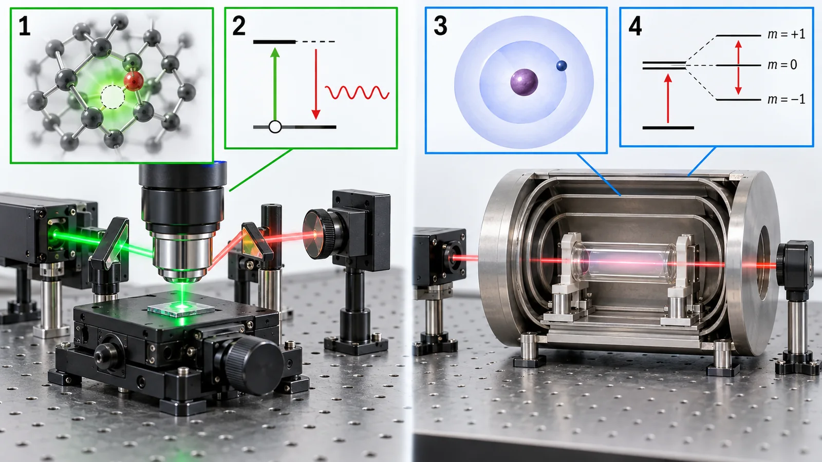
- What it does: it uses things with quantum properties, such as atoms and electron spins, as a “yardstick” to measure magnetic fields, time, gravity, temperature, current and more with great fineness. Unlike a quantum computer, it does not need many qubits; it works with anything from a single quantum object to a large collection
- Conclusion: many of these sensors have a long history, such as atomic clocks and SQUIDs (superconducting magnetometers), and some are in practical use. Others, such as NV centers in diamond, are at a stage where their sensitivity is orders of magnitude from the theoretical limit. “Quantum” does not automatically mean “better than classical”
- The most important point: the value of a quantum sensor depends on the combination of sensitivity (how small a quantity it can measure), stability, size and the environments where it works. A record value in a paper is not the same as performance in the field. The application examples here are mostly at the research-report stage, and we say so explicitly
It helps to know that a qubit can be drawn as an arrow from the centre of a sphere to its surface (north pole = 0, south pole = 1, tilted = superposition) and that the arrow gets blurred by its surroundings (decoherence). If this is new, the text explains what is needed. Middle-school science is enough for words like “magnetic field” and “frequency.”
Where this fits in the seriesRead this after our explainers on quantum computing fundamentals and on coherence and fidelity. Isotope-purified silicon is covered in our explainer on silicon spin qubits, and a review of isotope engineering that includes diamond is listed in its references. Optical components, lasers and detectors are covered in our explainers on semiconductor lasers, photodetectors and optical fiber, cryogenics in our explainer on cryogenics and control, and the overall materials and fabrication picture in our explainer on materials and fabrication for quantum computers. Quantum communication is in our explainer on quantum key distribution and quantum communication. AI-driven materials discovery is covered in our explainer on materials informatics.
- What quantum sensing is — quantum as a yardstick
- Reading sensitivity — sizes of magnetic fields and sensor noise (our calculation)
- NV centers in diamond — a defect that becomes a magnetometer
- Atomic magnetometers — measuring the brain's field with alkali vapor
- Atomic clocks and optical lattice clocks — time that measures height
- Gravimeters and atom interferometers — falling atoms that probe underground
- Examples of applications in materials, semiconductors and biology — avoiding exaggeration
- How it differs from, and resembles, quantum computing
- What we could not confirm, and a summary
- How to read evaluations and standards
- Glossary
- References (primary sources)
- Claim-to-source audit
Sourced = stated in a published source (with a link)
Our calculation = a value this article computed from stated assumptions
Not yet confirmed = plans, targets, items under review and so on
Our reading of what this means for materials is marked as commentary. Inference is shown in bold. Company announcements are treated as “company claims.”
Sensitivity values come from different measurement conditions (frequency band, integration time, sample size, environment), so placing them side by side does not rank them. A record value in a paper is a laboratory best, not performance that can be used in the field. The application examples are mostly at the research-report stage and do not imply product performance or adoption. No medical advice is given.
1. What quantum sensing is — quantum as a yardstick
First, an everyday sense
Think of a clock. A pendulum clock counts the swings of a pendulum to measure time. Now suppose every pendulum swings with exactly the same period. With no individual differences, a clock made anywhere would be the same clock. Atoms are close to this. Atoms of the same kind absorb light of exactly the same frequency (because their energy levels are values set by nature). An atomic clock uses that frequency as its “yardstick.”
This is the basic idea of quantum sensing. Things in the quantum world have discrete energy values, and the same values for the same kind of particle. If you read a slight shift in those values, you learn the influence of a magnetic field, gravity and so on.
A definition in words
The review by Degen and colleagues describes quantum sensing as the use of a quantum system, quantum properties or quantum phenomena to perform a measurement of a physical quantity, and lists SQUID and atomic-vapor magnetometers and atomic clocks as historical examples Sourced [Ref. 1]. They also divide quantum sensors into three types [Ref. 1].
- Type I: measuring with a quantum object that has discrete energy levels (spins, atoms, ions and so on)
- Type II: measuring with quantum coherence (wave-like superposition)
- Type III: using quantum entanglement to approach a sensitivity or precision that is impossible classically
The same review lists what a system needs to be a quantum sensor, in a form similar to the DiVincenzo criteria for quantum computers: (1) discrete energy levels, (2) it can be initialized and read out, (3) it can be manipulated coherently (and (4) it couples to the quantity to be measured) [Ref. 1]. The important point is that the same ingredients as a quantum computer are needed.
The arrow of a quantum sensor is like the hand of a clock. In a strong magnetic field the hand turns fast. By reading how many degrees it turned in a fixed time, you learn the strength of the field. The longer the hand can keep turning (the longer the coherence), the more a slight difference accumulates into a large difference in angle.
Limits of the analogy: the rotation of the arrow can be read out only probabilistically (one measurement gives only 0 or 1). So the same measurement is repeated many times and the angle is found statistically (next chapter).
Wrong: “quantum sensors cannot be used until quantum computers are practical.” In fact: a quantum sensor needs neither error correction nor many qubits; it works with a single atom or spin, or with a large collection of atoms. Atomic clocks have been used since the 1950s. Degen and colleagues call these historical examples of quantum sensing, and say that what is newer is that quantum systems are designed specifically for sensing and that entanglement is used as a resource Sourced [Ref. 1]. They are a different technology with a different level of maturity.
Quantum limits, and ordinary limits
When you measure with N identical quantum sensors, statistics improve the precision like 1/√N. This is called the standard quantum limit (SQL). The review by Degen and colleagues explains that this 1/√N scaling follows from the quantum Cramér-Rao bound, and that going beyond it requires states with quantum entanglement Sourced [Ref. 1]. With entanglement one can in theory approach 1/N (the Heisenberg limit). In experiments, however, noise (decoherence) is a major wall (our explanation).
2. Reading sensitivity — sizes of magnetic fields and sensor noise (our calculation)
What does “T/√Hz” mean?
The performance of a magnetometer is written as a “sensitivity” in units of T/√Hz (tesla per root hertz). It is a guide to the size of the magnetic field that cannot be told apart from noise after measuring for one second. The √Hz appears because noise averages down as the square root of time. If you lengthen the measurement time t (in seconds), the smallest measurable field becomes δB = η / √t (where η is the value in T/√Hz) (our explanation; for white noise).
For example, suppose you want to measure a field of 10 fT with a sensor of η = 1 pT/√Hz. The time needed is t = (η / δB)2 = (10−12 / 10−14)2 = 104 seconds, or about 2.8 hours Our calculation. If η is 1 fT/√Hz, the same 10 fT takes 0.01 seconds. A 1000-fold difference in sensitivity means a million-fold difference in measurement time. Barry and colleagues write that the roughly 1000-fold gap between NV ensemble sensors (pT/√Hz class) and SQUIDs or SERF magnetometers (fT/√Hz or below) corresponds to a roughly 106-fold increase in required averaging time, which rules out many envisioned applications Sourced [Ref. 3].
The brain's field (10 fT to 1 pT) is only about 108 to 1010 times smaller than the Earth's field (20 to 60 µT) (20 µT / 1 pT = 2 × 10⁷, 60 µT / 10 fT = 6 × 10⁹; Our calculation). So magnetically shielded rooms or ways of cancelling the background field are used. For example, the wearable magnetoencephalography system of Boto and colleagues combines quantum sensors with a way of nulling the background field Sourced [Ref. 9].
3. NV centers in diamond — a defect that becomes a magnetometer
What an NV center is
Diamond is a crystal in which carbon atoms are lined up regularly. In it there is a defect in which one carbon atom has been replaced by nitrogen (N) and the neighboring carbon atom is missing, leaving a vacancy (V). This is called an NV center (nitrogen-vacancy center). Barry and colleagues describe it as a point defect made of a substitutional nitrogen fixed next to a vacancy within the rigid carbon lattice Sourced [Ref. 3]. There are three charge states, and the negatively charged NV− is the one used for quantum sensing [Ref. 3].
This defect is like an artificial atom trapped inside diamond. According to Barry and colleagues, the ground state of NV− is a spin-1 triplet with long spin lifetimes at room temperature (a longitudinal relaxation time T1 of about 6 ms is typical, and coherence times T2 up to a few ms are achievable) [Ref. 3].
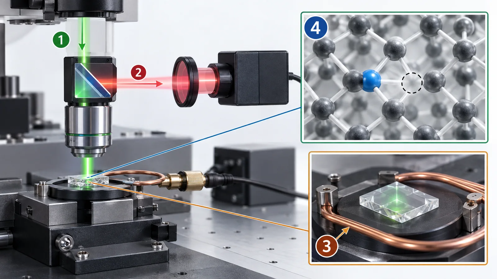
View original SVG, values and sources
Original SVG reference: Conceptual diagram (vector drawing). Left: a sketch of the diamond crystal, with an NV center where a nitrogen sits next to a vacancy. Right: the flow in which a green laser aligns the spin into ms = 0, microwaves rotate the state, and the brightness of the fluorescence reads it out (based on the description in the review by Barry and colleagues). The gap between ms = 0 and ±1 is about 2.87 GHz, and a magnetic field splits the ±1 levels [Ref. 3]. The relative heights of the levels are illustrative.
Align with light, rotate with microwaves, read with light
The spin of an NV center can be handled with light and microwaves alone. When a green laser (about 532 nm) shines on it, the spin is aligned into a definite state (ms = 0) (initialization), and the brightness of the red fluorescence differs with the spin state. Microwaves (around 2.87 GHz) rotate the state, and the fluorescence brightness reads it out Sourced [Ref. 3]. When a magnetic field is applied the energy levels split, so the microwave frequency at which the fluorescence dips gives the field (our explanation). The energy levels of an NV center are sensitive to magnetic fields, electric fields, strain and temperature, so one defect works as a multi-purpose sensor [Ref. 3]. In temperature, the zero-field splitting D changes by about −74 kHz/K [Ref. 3].
The advantage is that it works at room temperature, atmospheric pressure and low magnetic fields, and needs no cryogenic cooling, vacuum system or tesla-scale magnet. Barry and colleagues note that diamond is chemically inert and biocompatible, and that the sensor can be placed within about 1 nm of what is to be measured Sourced [Ref. 3].
How sensitive is it? — single and ensemble, and the gap to the theoretical limit
According to Wolf and colleagues, the room-temperature magnetic-field sensitivity of a single NV center is limited to about 10 nT/√Hz. With an ensemble of N centers, the sensitivity improves in proportion to √N. They used an ensemble of 1011 NV centers and reached the photon-shot-noise-limited 0.9 pT/√Hz (effective sensor volume 8.5 × 10⁻⁴ mm3), which they describe as the best diamond magnetometer sensitivity so far Sourced [Ref. 4].
Let us do a simple calculation. 10 nT/√Hz / √(1011) = 10−8 / 3.2 × 105 = about 32 fT/√Hz. The measured 0.9 pT/√Hz is about 28 times larger (worse) than this simple estimate Our calculation (a rough comparison between experiments with different numbers and conditions, so only a guide). Barry and colleagues write that present NV ensemble devices have sensitivities orders of magnitude away from theoretical limits, and that the most promising avenues are the spin dephasing time, the readout fidelity and the properties of the host diamond material Sourced [Ref. 3]. They also state that while SQUIDs and SERF magnetometers reach fT/√Hz or below, NV ensembles are at the pT/√Hz level, a roughly 1000-fold gap [Ref. 3].
Wrong: “an NV center is a quantum sensor, so its magnetic sensitivity is the best.” In fact: the strengths of the NV center are not sensitivity but spatial resolution, room-temperature operation, small size, and the ability to bring the sensor close to the object. In pure sensitivity (T/√Hz), SQUID and SERF magnetometers are about 1000 times better, as the NV review itself says [Ref. 3]. Which one fits depends on what you want to measure (the field in a small region, or a weak field over a large region).
Materials set the performance — nitrogen and 13C in diamond
The sensitivity of an NV ensemble is set by the spin dephasing time T2*, and T2* is set by impurities and isotopes in the diamond (the review by Barry and colleagues) [Ref. 3]. There are two major factors.
- Substitutional nitrogen (nitrogen that did not become an NV): a magnetic noise source. Barry and colleagues express the dephasing of an NV ensemble by nitrogen with a coefficient of 101 ms−1 ppm−1 [Ref. 3].
- 13C (a carbon isotope with a nuclear spin): natural diamond contains 13C at 10,700 ppm (about 1.1%), which shifts the phase of the NV electron spin [Ref. 3]. This plays exactly the role of 29Si in silicon (see our explainer on silicon spin qubits).
Barry and colleagues give the limit that 13C sets on the dephasing time as 1/T2*(13C) = A13C × [13C], with coefficient A13C ≈ 0.100 ms−1 ppm−1 Sourced [Ref. 3]. Using this, for natural 13C (10,700 ppm) the upper limit of T2* is about 0.93 µs, and with 12C purified to 99.999% (13C at 10 ppm) it is about 1 ms Our calculation. Barry and colleagues also say that T2*(13C) for natural-abundance diamond is about 1 µs [Ref. 3]. Isotope purification raises the limit more than a thousandfold.
As an example of 12C purification, Barry and colleagues note that Teraji and colleagues used methane with 99.999% 12C (13C of 10 ppm or less) to obtain CVD diamond whose 12C concentration measured by SIMS was 99.998% [Ref. 3]. The same review says that such isotopically enriched methane is 103 to 104 times more expensive than natural-abundance methane, and that 13C can also get in from other carbon sources in the CVD chamber Sourced [Ref. 3]. An overview of isotope control in diamond and silicon is given in the review by Itoh and Watanabe [Ref. 18].
In an NV ensemble sensor, more NV centers give a larger signal, but making NV centers needs nitrogen, and more nitrogen shortens T2*. For example, Barry and colleagues estimate that the nitrogen concentration at which substitutional nitrogen and natural 13C contribute equally is about 10.6 ppm [Ref. 3]. So you must control the nitrogen concentration (ppm), the fraction of nitrogen that became NV, the 13C concentration, crystal strain and the surface condition at the same time. The table of Barry and colleagues summarizes, for example, that CVD synthesis makes dimensions and concentrations easy to control but can introduce strain and impurities, that HPHT synthesis gives less strain and fewer defects but makes doping harder to control, and that terminating the surface with suitable elements can stabilize the charge state of NV centers near the surface [Ref. 3]. For a materials engineer, this is a field where crystal growth, isotope feedstock and surface treatment directly become the sensor's performance (our commentary).
4. Atomic magnetometers — measuring the brain's field with alkali vapor
How it works — atoms in a glass container become tiny compasses
An atomic magnetometer puts vapor of an alkali metal such as rubidium or cesium in a glass cell. Kominis and colleagues describe it as detecting the Larmor spin precession (turning) of optically pumped atoms Sourced [Ref. 6]. The flow is as follows (our explanation).
- A circularly polarized laser (the pump beam) aligns the spins of the vapor atoms in the same direction
- In a magnetic field, the aligned spins begin to turn
- A second laser (the probe beam) passes through the vapor, and the change in its polarization shows how the spins are turning
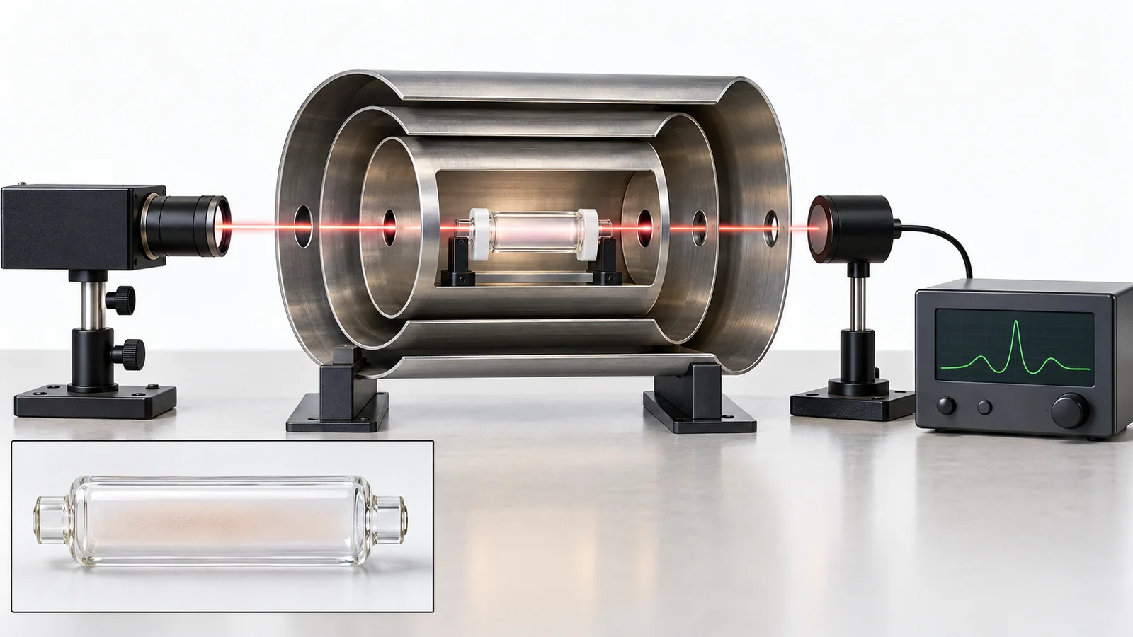
View original SVG, values and sources
Original SVG reference: Conceptual diagram (vector drawing). A concept drawing of an atomic magnetometer in which the pump beam aligns the alkali-vapor atoms in a glass cell, a magnetic field turns the spins, and the probe beam and detector read them. The real layout depends on the scheme (SERF, Larmor, zero-field and others).
SERF magnetometers — the condition that nearly removes the noise
When atoms collide with each other and their spins are scrambled (spin-exchange relaxation), sensitivity drops. In the SERF (spin-exchange relaxation-free) regime this relaxation can be removed. Kominis and colleagues report that a SERF magnetometer reached 0.54 fT/√Hz with a measurement volume of only 0.3 cm3, and that their analysis puts the fundamental limit of the device below 0.01 fT/√Hz Sourced [Ref. 6]. However, Budker and Romalis explain that the SERF regime holds only for magnetic fields below about 10 nT, and that in a field such as the Earth's, a SERF magnetometer is used as a null detector with external feedback [Ref. 7]. That is why magnetic shielding or a way of cancelling the background field is needed.
A SQUID works at 4 K (liquid-helium temperature) and has a sensitivity of about 1 fT/√Hz, but it needs cooling. Kominis and colleagues write that atomic magnetometers could reach similar sensitivity without cryogenic cooling, opening new applications such as non-invasive mapping of the cortex [Ref. 6]. Budker and Romalis also list no need for cryogenic cooling and the potential for miniaturization as advantages of atomic magnetometers [Ref. 7].
When atoms hit the container wall, they lose the spin direction they were aligned in. So the wall must be made gentle on atoms. As ways to reduce wall relaxation, Budker and Romalis name coating the inside of the wall with materials such as paraffin, which have long hydrocarbon chains, or filling the cell with another gas (a buffer gas) that slows the atoms' diffusion to the wall [Ref. 7].
As a direction toward mass-produced, low-cost small magnetometers, Budker and Romalis describe an integrated sensor in which a VCSEL laser, an alkali vapor cell, optics and a detector are made with the wafer-production techniques of the semiconductor industry. At that time (2007), a grain-of-rice-sized integrated sensor had shown a sensitivity of 50 pT/√Hz Sourced [Ref. 7]. Shah and colleagues demonstrated a subpicotesla atomic magnetometer using a microfabricated vapor cell (as given in the title) [Ref. 8]. From the materials side, this is a field where glass-silicon bonding, filling and sealing of alkali metal, and the heat resistance and uniformity of the wall coating decide the sensor's sensitivity and lifetime (our explanation; glass and fiber materials are covered in our explainer on optical fiber).
Measuring the brain's field without cooling
Boto and colleagues reported a wearable magnetoencephalography (MEG) system that can be worn like a helmet, combining quantum sensors (optically pumped atomic magnetometers) with a way of cancelling the background field. They state that subjects could move naturally, for example nodding the head or playing with a ball, while brain activity was measured with millisecond resolution Sourced [Ref. 9]. Conventional SQUID-based MEG required the head to be held still. Declaration of competing interests: the paper states that one of its authors is the founding director of the company that sells the atomic magnetometers used, and that the company built the sensors and advised on the system design [Ref. 9]. Whether wearable MEG becomes practical still needs to be verified Not yet confirmed.
5. Atomic clocks and optical lattice clocks — time that measures height
How an atomic clock works
The first practical caesium atomic clock was built in 1955 (as stated at the opening of the paper by Takamoto and colleagues) Sourced [Ref. 11]. The definition of the second is tied to a microwave transition of the caesium atom; according to BIPM (the International Bureau of Weights and Measures) it is fixed by the microwave frequency characteristic of the Cs atom (ΔνCs) [Ref. 34]. In their 2005 paper, Takamoto and colleagues write that the fractional uncertainty of this realization of the second is about 10−15 [Ref. 11].
The principle resembles a pendulum clock (our explanation). The frequency of a laser or microwave source is kept matched to a definite frequency that the atom absorbs, and the oscillations at that frequency are counted to make time. Every atom has the same frequency, so atoms give the same yardstick.
Optical lattice clocks — counting the oscillation of light, more finely
The frequency of light is much higher than that of microwaves (it oscillates faster), so the same time can be divided more finely (our explanation). To count the oscillations of light, a technology called the optical frequency comb links optical and radio frequencies [Ref. 11]. The group of Katori reported an optical lattice clock in 2005. In this scheme, many atoms are trapped in a “lattice” made by a standing wave of light and used as the quantum reference, with the potential to combine the accuracy of trapped ions with the stability of neutral atoms Sourced [Ref. 11].
Progress since has been large. In 2022, Bothwell and colleagues reduced the fractional frequency measurement uncertainty to 7.6 × 10⁻²¹, enough to measure the gravitational redshift within a single millimetre-scale sample of ultracold strontium Sourced [Ref. 13]. The review of optical clocks organizes in detail the measurement precision and systematic uncertainty of optical clocks that use trapped single ions and many neutral atoms [Ref. 10].
A time shift is a height difference — our calculation
According to general relativity, a clock at a higher place runs faster than a clock at a lower place (gravitational redshift). The fractional frequency shift for a height difference Δh is approximately Δf/f = gΔh / c2 (a general approximation; our explanation). Putting in g = 9.80665 m/s2 and c = 299,792,458 m/s gives about 1.1 × 10⁻¹⁸ for 1 cm, about 1.1 × 10⁻¹⁶ for 1 m and about 4.9 × 10⁻¹⁴ for 450 m Our calculation. So a clock with an uncertainty at the 10−18 level can detect a height difference of about 1 cm as a time shift. Takamoto and colleagues make the same point [Ref. 12].
In 2020, Takamoto and colleagues built two transportable optical lattice clocks, placed them at the bottom and top of Tokyo Skytree (a height difference of 450 m), and made a frequency comparison with 18-digit precision. They write that the gravitational redshift was tested at (1.4 ± 9.1) × 10−5 relative to the prediction, an order of magnitude better than earlier ground-based clock comparisons Sourced [Ref. 12]. The same paper says optical clocks that can resolve centimetres are technically ready for field applications such as monitoring changes of geopotential caused by volcanoes or crustal deformation, and defining the geoid [Ref. 12].
How fast a clock runs changes slightly with the strength of gravity (height). So if you place two high-precision clocks at different locations and compare how fast they run, you learn the difference in “gravitational potential” between the two places, which is in effect the height difference. A tool for measuring time also becomes a tool for measuring height. Geodetic applications of this are at the research stage (Takamoto and colleagues list them as possibilities [Ref. 12]) Not yet confirmed.
Changing the definition of the second — a plan versus an achievement
According to BIPM, some optical frequency standards have reached systematic uncertainties two orders of magnitude smaller than caesium fountain clocks. The roadmap updated by the CCTF in 2025 treats 2030 as the decisive milestone, and at the CGPM in 2026 progress is to be reviewed and a draft resolution on continued work toward 2030 considered Sourced [Ref. 34]. The conditions for redefinition include an improvement of accuracy by 10 to 100 times, continuity with the caesium definition, continuous availability, and acceptability to national metrology institutes [Ref. 34]. We could not confirm the outcome of the 2026 CGPM. Redefining the second is a matter planned to be decided in 2030 Not yet confirmed.
An optical lattice clock consists of lasers that cool the atoms, lasers that make the lattice, an extremely stable laser that probes the atomic resonance, an optical frequency comb, an ultrahigh-vacuum chamber and magnetic shielding (our explanation; the technical ingredients are organized in the review by Ludlow and colleagues [Ref. 10]). On the materials side, outgassing of vacuum-chamber materials, coatings on optical windows, and the materials of laser sources, modulators and fibers decide stability and reliability. In the direction of miniaturization, a chip-scale atomic clock using a microfabricated vapor cell was reported in 2004 (as given in the title) [Ref. 33]. Many of these parts overlap with the materials covered in our explainers on semiconductor lasers, thin-film lithium niobate, optical fiber and photodetectors.
6. Gravimeters and atom interferometers — falling atoms that probe underground
Using atoms as waves
In the quantum world, an atom is both a particle and a wave. An atom interferometer takes a cooled cloud of atoms and applies laser pulses three times, splitting the atomic wave in two and then recombining it. A phase difference due to gravity and other effects builds up along the two paths, and the interference seen on recombination reveals the acceleration (gravity). In 1999, Peters and colleagues used an atom interferometer based on a fountain of laser-cooled atoms to measure the acceleration of gravity g, and obtained an absolute uncertainty of Δg/g ≈ 3 × 10⁻⁹. They describe this as a million-fold improvement in absolute accuracy over earlier atom-interferometer experiments, and report that a macroscopic glass object falling in a Michelson-interferometer gravimeter fell with the same acceleration as a caesium atom to within 7 parts in 109 Sourced [Ref. 14].
Multiplying Δg/g ≈ 3 × 10⁻⁹ by g ≈ 9.8 m/s2 gives about 2.9 × 10⁻⁸ m/s2 (about 2.9 µGal) Our calculation.
Finding an underground tunnel in the field
In 2022, Stray and colleagues reported field-survey results from a quantum gravity-gradient sensor. The instrument is designed to suppress micro-seismic and laser noise, temperature and magnetic-field variations, and instrument tilt. It reached a statistical uncertainty of 20 E (1 E = 10−9 s−2), carried out a survey with 0.5 m spatial resolution along an 8.5 m line, and detected a 2 m tunnel with a signal-to-noise ratio of 8. Using Bayesian inference, they determined the centre horizontally to ±0.19 m and the centre depth as 1.89 m (−0.59/+2.3 m) Sourced [Ref. 15]. The authors say that mapping aquifers, archaeology, determining soil properties, and reducing the risk of unforeseen ground conditions in infrastructure construction could be applications [Ref. 15].
The perspective by Bongs and colleagues says that atom interferometers are moving out of the laboratory to be used as ultraprecise quantum sensors in metrology, geophysics, space, civil engineering, oil and mineral exploration, and navigation, and discusses the scientific and technological challenges [Ref. 16].
Wrong: “atomic gravimeters have become the standard.” In fact: in the international comparison of absolute gravimeters (CCM.G-K2.2023, held in August and September 2023 at NIST in the United States), of 30 absolute gravimeters, 27 were conventional free-fall instruments (FG5 and FG5X), 1 was an NIM-3A, and 2 were atom gravimeters (both from China). The report of the BIPM working group says that in the key-comparison part (15 instruments from national metrology institutes and similar bodies) all the instruments agreed excellently Sourced [Ref. 36]. Atom gravimeters may be strong in field, mobile and long-duration measurements, but they are still a small minority among the instruments in international comparisons (our explanation).
Atom interferometers and optical clocks run on ultrahigh-vacuum chambers, low-outgassing metals, optical windows, lasers and magnetic shielding. Stray and colleagues write that their design suppresses micro-seismic and laser noise, temperature and magnetic-field variations, and tilt [Ref. 15], which are also questions of thermal expansion, magnetism and mechanical stability of materials (our explanation). The quantum part is the atoms, but for a materials engineer the key point is that much of the real performance is decided by the classical materials around them.
7. Examples of applications in materials, semiconductors and biology — avoiding exaggeration
Here we introduce applications of quantum sensors while stating what stage each report is at. “Reported” and “in use in the field” are different things. The studies that opened up nanoscale magnetic sensing with a single NV center are the 2008 papers by Maze et al., Balasubramanian et al. and Taylor et al. (as given in the titles) Sourced [Refs. 28, 29, 30]. A review for physics and biology is given by Schirhagl et al. [Ref. 17].
| Field | Example application | What was reported (source) | Stage and cautions |
|---|---|---|---|
| Semiconductors | Imaging current in an integrated circuit (NV ensemble) | Nowodzinski et al. (2015): over a 50 × 200 µm2 region of an IC carrying mA-range current, measured the three components of the magnetic field with sub-micron resolution. Acquisition time about 10 s, faster than scanning with SQUID or GMR. Measured at room temperature and atmospheric pressure with a standard optical-microscope setup [Ref. 22] Sourced | An early laboratory experiment. The paper calls them early experiments not optimized for ICs. It does not imply product evaluation or adoption |
| Materials, geoscience, biology | Quantum diamond microscope (a sample on a layer of NV centers; a 2D map of the field) | Levine et al. (review): a dense layer of NV centers near the surface of a transparent diamond chip, with fluorescence measured across the whole surface at once, gives a wide-field magnetic image. Example applications in geoscience, biology and materials science are summarized [Ref. 23] Sourced | A review. The examples are research reports |
| Materials (superconductors) | Observing vortices (quantized flux) in a superconductor | Thiel et al. (2016): scanning a single NV at cryogenic temperature, quantitatively imaged Pearl vortices in YBa2Cu3O7−δ with a sensor-to-sample distance of about 10 nm [Ref. 24] Sourced | A cryogenic research report |
| Biology | Magnetic image of living bacteria | Le Sage et al. (2013): imaged living magnetotactic bacteria on an NV diamond chip at 400 nm resolution, reconstructing the field made by chains of magnetic nanoparticles [Ref. 25] Sourced | A laboratory demonstration |
| Biology | Temperature inside living cells | Kucsko et al. (2013): with NV centers in nanodiamonds, detected temperature changes as small as 1.8 mK in ultrapure samples, with spatial resolution down to 200 nm. Introduced nanodiamonds and gold nanoparticles into a human embryonic fibroblast to control and map temperature gradients inside the cell [Ref. 26] Sourced | A demonstration in cultured cells. Medical applications need separate study |
| Biology | Magnetic field of a single neuron's action potential | Barry et al. (2016): measured the magnetic field of action potentials with NV centers on single neurons excised from a marine worm and a squid. Single-neuron action potentials were also measured from outside live marine worms for extended periods [Ref. 27] Sourced | A demonstration in invertebrates. We have not confirmed applications in humans |
| Neuroscience | Wearable magnetoencephalography (atomic magnetometers) | Boto et al. (2018): a helmet-type system combining quantum sensors with cancellation of the background field. Brain activity measured with millisecond resolution during natural movement [Ref. 9] Sourced | A research report. One author is the founder of the sensor-selling company, which was involved (stated in the paper). We have not confirmed clinical performance |
| Civil engineering, ground | Detecting an underground tunnel (quantum gravity-gradient sensor) | Stray et al. (2022): in the field, detected a 2 m tunnel along an 8.5 m line with a signal-to-noise ratio of 8 [Ref. 15] Sourced | A field demonstration. We have not confirmed wide-area surveys or comparisons with other instruments |
| Geodesy | Measuring height differences with clocks | Takamoto et al. (2020): tested the 450 m height difference at Tokyo Skytree with two transportable optical lattice clocks [Ref. 12] Sourced | A demonstration. Monitoring volcanoes and crustal deformation are possibilities named by the authors (Not yet confirmed) |
The table is our own organization (Our calculation). The “Stage” column is our reading of each paper's description, not a judgment of whether a product exists or how mature it is. No individual medical, food or safety advice is given.
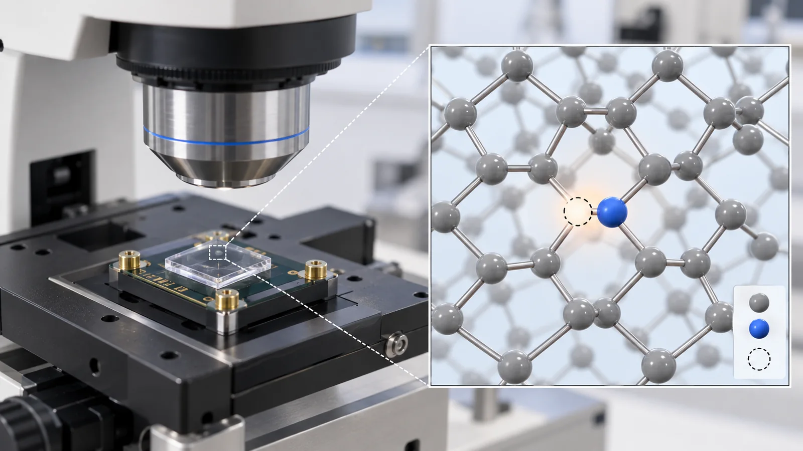
The strength of the NV magnetic sensor is not sensitivity but that it can be brought to within nanometres of the sample (Barry and colleagues say about 1 nm [Ref. 3]; Thiel and colleagues imaged vortices at about 10 nm [Ref. 24]). Magnetic fields fall off rapidly with distance, so getting close lets you measure the field of a small region even with modest sensitivity. In materials and devices, this means a possible tool to examine current distribution, magnetism distribution and local temperature non-destructively (our explanation). We have not confirmed practical use in semiconductor failure analysis.
8. How it differs from, and resembles, quantum computing
| Aspect | Quantum computer | Quantum sensor | What they share, and cautions |
|---|---|---|---|
| Purpose | Obtain the answer to a computation using superposition, interference and entanglement | Measure a physical quantity using a quantum system as the yardstick (the definition of Degen et al.) [Ref. 1] | Both use quantum superposition and readout |
| Number of qubits needed | Thought to need many for practical use (for error correction) | Works with one to many. Type III (using entanglement) needs several [Ref. 1] | Some quantum sensors, such as atomic clocks, are already in use without waiting for quantum computers |
| Errors and noise | The goal is to “remove” noise. Error correction is the central issue | The goal is to “pick up” the influence of the quantity to measure. Other noise lowers sensitivity | In both, coherence time sets performance |
| Meaning of the “quantum advantage” | Speed of computation compared with the best classical method (quantum advantage) | Differences in sensitivity, precision, size and usable environment compared with classical sensors. Relation to theoretical limits (SQL, Heisenberg limit) [Refs. 1, 19] | It cannot simply be said that “quantum is better” (the NV example, Chapter 3) |
| Shared materials and parts | The review says the NV center in diamond is a basis for quantum metrology, information processing and communications [Ref. 2]. Isotope-purified materials (silicon, diamond) [Ref. 18] | The same NV centers and isotope-purified diamond. Lasers, optics, photodetectors, vacuum, and cryogenics (for SQUIDs) | Purity, isotope ratio and interface quality set performance in both (our explanation) |
| Use of non-classical light | Photonic quantum computers and others | Examples using squeezed light (light with reduced quantum noise) in gravitational-wave detectors: GEO 600 (operating beyond the quantum shot-noise limit, as given in the title) and LIGO (improved sensitivity, as given in the title) [Refs. 31, 32] Sourced | The idea of “designing” quantum noise to reduce it is shared |
| Maturity | Error correction with many qubits is still ahead | Atomic clocks and SQUIDs are mature. NV centers, atomic magnetometers, optical lattice clocks and atom interferometers include a mix of report stages | The stage has to be checked for each application (Chapter 7) |
The table is our own organization (Our calculation). It does not argue which is better.
The “quantum advantage” of a quantum computer means being faster than the best classical method at a particular computation. For quantum sensors, the nearest idea is “sensitivity beyond classical limits.” For example, using entanglement to go beyond the standard quantum limit 1/√N of N sensors (approaching the Heisenberg limit of 1/N) [Refs. 1, 19]. But most practical quantum sensors are not at the stage of beating such limits; their value is that using a quantum yardstick lets them measure more compactly, at room temperature, or without calibration compared with classical methods (our explanation). When you compare sensitivity numbers, check whether they are compared with the best classical sensor under the same conditions.
9. What we could not confirm, and a summary
What we could not confirm
- The outcome of the 2026 CGPM (which discusses progress on redefining the second): on BIPM's page we could confirm the planned meeting and the roadmap (2030 as the decisive milestone), but not the outcome of the meeting [Ref. 34].
- Records of NV magnetometer sensitivity since 2020: we stayed with the picture in the review by Barry and colleagues (2020) and did not comprehensively check later records.
- Performance, sales and adoption of quantum sensor products: we did not check company product specifications or market sizes against primary sources, and do not state them.
- Practical industrial use of NV sensors, such as semiconductor failure analysis: what we could confirm is an early laboratory experiment of 2015 [Ref. 22].
- Field use of quantum sensors that use entanglement (Type III): not confirmed.
- Standards specific to quantum sensing: not confirmed (Chapter 10).
- Domestic research programs and company efforts: not covered in this article (not checked).
- Quantum sensing measures with a quantum system as the yardstick. It works through the same three steps as a quantum computer, “initialize, act, read out,” and can be used with one object or many. Some, such as atomic clocks, are in use without waiting for quantum computers Sourced
- Sensitivity is written in T/√Hz or similar, and a 1000-fold gap means a million-fold gap in measurement time. NV ensembles are at the pT/√Hz level, about 1000 times worse than SQUIDs or SERF (fT/√Hz and below), and orders of magnitude from the theoretical limit Sourced / Our calculation
- Materials decide performance. Purifying the 13C of diamond (about 1.1% in nature) raises the upper limit of the dephasing time from about 1 µs to about 1 ms (the same idea as isotope purification of silicon). For vapor cells, wall coatings and wafer-fabrication techniques are the key Sourced / Our calculation
- Optical lattice clocks can also measure height differences. Clocks at the 10−18 level can resolve a height difference of about 1 cm (about 1.1 × 10⁻¹⁸). Redefining the second is a discussion heading toward 2030 Sourced / Our calculation / Not yet confirmed
- Read applications by checking their stage. Imaging current in an IC, temperature inside cells, magnetic fields of single neurons, an underground tunnel and clock comparison at Skytree are all at the research-report or demonstration stage. In the international comparison of absolute gravimeters, 2 of 30 were atom gravimeters Sourced
10. How to read evaluations and standards
The performance of a quantum sensor is measured by sensitivity (how small a quantity it can measure; T/√Hz and so on), stability and uncertainty (fractional uncertainty and Allan deviation for clocks), accuracy (the correctness of absolute values; for example international comparisons of gravimeters), spatial resolution, size and the environments where it works. No single number tells the whole story. On the standards side there are definitions of frequency and time stability (IEEE 1139-2022), international comparisons of absolute gravimeters (BIPM), and the definition of the second (SI). But we could not confirm any evaluation standard specific to quantum sensing (checked 16 October 2026).
| What is evaluated | Representative benchmark or method (name, source) | Standards and guidance (ISO/IEC, IEEE, BIPM and others) | Cautions in reading |
|---|---|---|---|
| Magnetic-field sensitivity | Noise density (T/√Hz). SQUID about 1 fT/√Hz, SERF 0.54 fT/√Hz, NV ensemble 0.9 pT/√Hz [4, 6] Sourced | Not confirmed | The value changes with frequency band, integration time and sensor volume. A 1000-fold sensitivity gap is a million-fold gap in measurement time [3] |
| Fundamental limits | Standard quantum limit (1/√N) and Heisenberg limit (1/N) (Degen et al., Giovannetti et al.) [1, 19] Sourced | Not confirmed | Many practical sensors are limited by technical noise short of this limit (our explanation) |
| Frequency and time stability | Fractional uncertainty (Sr optical lattice clock, 7.6 × 10⁻²¹) [13]. Allan deviation and the like | IEEE 1139-2022 “Standard Definitions of Physical Quantities for Fundamental Frequency and Time Metrology — Random Instabilities” (published 8 December 2022, active, replacing the 2008 edition; it covers frequency, phase and amplitude instabilities and their time-domain deviations) [35] Sourced | We did not check the text of the standard and do not describe its definitions |
| Definition of the second | Comparison of optical frequency standards (BIPM) | The SI second is defined by the microwave frequency of caesium. Redefinition is being considered toward 2030 [34] Sourced / Not yet confirmed | The outcome of the 2026 CGPM is not confirmed |
| Accuracy of absolute gravimeters | International comparison CCM.G-K2.2023 (August to September 2023, NIST; 30 instruments from 27 institutes, of which 2 were atom gravimeters) [36] Sourced | A key comparison led by BIPM | In the key-comparison part (15 instruments) all agreed well. It does not mean atom gravimeters have become the standard instrument |
| Terminology and scope | — (a terminology standard, not an evaluation) | ISO/IEC 4879:2024 (a vocabulary for quantum computing, not for quantum sensing) [37]. The scope of ISO/IEC JTC 3 includes quantum metrology and detectors (one standard published, twelve under development) [38] Sourced | We did not check the text of the standards. We could not confirm a standard specific to sensing |
The table is our own organization (Our calculation). Numbers in brackets are reference numbers. Numbers, titles and status of standards and BIPM documents were checked on the official pages (16 October 2026). Standards texts are paywalled, so we limit ourselves to titles and scope.
Cautions in reading (for materials engineers)
- Sensitivity is a number with conditions: it changes with frequency band, integration time, sensor volume and environment (whether magnetic shielding is used). Even the same “pT/√Hz” cannot be compared if the premises differ
- A record in a paper and performance in the field are different: the 0.9 pT/√Hz of Wolf and colleagues is one laboratory's record, and the review by Barry and colleagues says that typical devices are orders of magnitude away from the theoretical limit [3, 4]
- Check the company's involvement: where a company that sells the sensor is involved, as in the paper of Boto and colleagues, competing interests are stated in the paper [9]. The performance of company products must be checked against primary sources
- Plans and achievements are different: redefining the second (a discussion toward 2030) and geodetic applications of optical clocks are Not yet confirmed. Standards are mostly recommendations, not requirements
11. Glossary
- Quantum sensing
- Measuring a physical quantity with a quantum system, quantum properties or quantum phenomena.
- Quantum sensor
- A system with discrete energy levels that is initialized, manipulated and read out to serve as a yardstick.
- Coherence
- The state of a quantum object (the direction of its arrow) staying undisturbed by its surroundings.
- Standard quantum limit (SQL)
- The limit at which precision improves as 1/√N with N independent sensors.
- Heisenberg limit
- The 1/N limit that entanglement can approach.
- T/√Hz
- The unit of magnetometer sensitivity. A guide to the smallest field distinguishable in 1 s.
- NV center
- A defect in diamond in which a nitrogen sits next to a vacancy. It has spin and can measure magnetic fields and more.
- Optically detected magnetic resonance (ODMR)
- Initialize with light, rotate with microwaves, and read the change in fluorescence.
- T2*
- The time over which the phase stays aligned. The longer it is, the smaller the field differences you can see.
- 13C / 12C
- Carbon isotopes in diamond. 13C has a nuclear spin and is a noise source for NV.
- Substitutional nitrogen
- Nitrogen sitting at a carbon site. Nitrogen that did not become an NV is a magnetic noise source.
- CVD / HPHT
- Ways to synthesize diamond (chemical vapor deposition / high pressure, high temperature).
- Atomic magnetometer
- A sensor that measures a magnetic field from the turning of the atomic spins of an alkali vapor.
- Optical pumping
- Aligning the direction of atomic spins with circularly polarized light.
- SERF
- Spin-exchange relaxation-free regime. Very high sensitivity is possible at fields below about 10 nT.
- SQUID
- A superconducting quantum interference device. A magnetometer that works at 4 K.
- Magnetoencephalography (MEG)
- A device that measures the very weak magnetic fields made by neural activity in the brain.
- Optical lattice clock
- A clock that traps many atoms in a lattice made by a standing wave of light and counts the frequency of light.
- Optical frequency comb
- A technology that links optical and radio frequencies.
- Gravitational redshift
- The effect that a clock at a higher place runs faster. Δf/f = gΔh/c2.
- Fractional uncertainty
- A frequency error divided by the frequency. A guide to clock accuracy.
- Allan deviation
- A time-domain measure of frequency stability.
- Atom interferometer
- A device that splits and recombines an atomic wave and measures gravity and more from the phase difference.
- Gravity gradiometer
- A device that measures the difference of gravity between two points. The unit E (eotvos) is 10−9 s−2.
- Squeezed light
- Light with the quantum noise in one quantity reduced. Used in gravitational-wave detectors.
- CCM / ICAG
- BIPM's consultative committee for mass and related quantities, and the international comparison of absolute gravimeters it leads.
12. References (primary sources)
- Degen C. L., Reinhard F., Cappellaro P. "Quantum sensing", Rev. Mod. Phys. 89, 035002 (2017), DOI 10.1103/RevModPhys.89.035002 (arXiv:1611.02427) — doi.org/10.1103/RevModPhys.89.035002
- Doherty M. W. et al. "The nitrogen-vacancy colour centre in diamond", Physics Reports 528, 1–45 (2013), DOI 10.1016/j.physrep.2013.02.001 — doi.org/10.1016/j.physrep.2013.02.001
- Barry J. F. et al. "Sensitivity optimization for NV-diamond magnetometry", Rev. Mod. Phys. 92, 015004 (2020), DOI 10.1103/RevModPhys.92.015004 (arXiv:1903.08176) — doi.org/10.1103/RevModPhys.92.015004
- Wolf T. et al. "Subpicotesla Diamond Magnetometry", Phys. Rev. X 5, 041001 (2015), DOI 10.1103/PhysRevX.5.041001 (arXiv:1411.6553) — doi.org/10.1103/PhysRevX.5.041001
- Balasubramanian G. et al. "Ultralong spin coherence time in isotopically engineered diamond", Nature Materials 8, 383–387 (2009), DOI 10.1038/nmat2420 — doi.org/10.1038/nmat2420
- Kominis I. K. et al. "A subfemtotesla multichannel atomic magnetometer", Nature 422, 596–599 (2003), DOI 10.1038/nature01484 — doi.org/10.1038/nature01484
- Budker D., Romalis M. "Optical magnetometry", Nature Physics 3, 227–234 (2007), DOI 10.1038/nphys566 (arXiv:physics/0611246) — doi.org/10.1038/nphys566
- Shah V. et al. "Subpicotesla atomic magnetometry with a microfabricated vapour cell", Nature Photonics 1, 649–652 (2007), DOI 10.1038/nphoton.2007.201 — doi.org/10.1038/nphoton.2007.201
- Boto E. et al. "Moving magnetoencephalography towards real-world applications with a wearable system", Nature 555, 657–661 (2018), DOI 10.1038/nature26147 — doi.org/10.1038/nature26147
- Ludlow A. D., Boyd M. M., Ye J., Peik E., Schmidt P. O. "Optical atomic clocks", Rev. Mod. Phys. 87, 637–701 (2015), DOI 10.1103/RevModPhys.87.637 — doi.org/10.1103/RevModPhys.87.637
- Takamoto M., Hong F.-L., Higashi R., Katori H. "An optical lattice clock", Nature 435, 321–324 (2005), DOI 10.1038/nature03541 — doi.org/10.1038/nature03541
- Takamoto M. et al. "Test of general relativity by a pair of transportable optical lattice clocks", Nature Photonics 14, 411–415 (2020), DOI 10.1038/s41566-020-0619-8 — doi.org/10.1038/s41566-020-0619-8
- Bothwell T. et al. "Resolving the gravitational redshift across a millimetre-scale atomic sample", Nature 602, 420–424 (2022), DOI 10.1038/s41586-021-04349-7 — doi.org/10.1038/s41586-021-04349-7
- Peters A., Chung K. Y., Chu S. "Measurement of gravitational acceleration by dropping atoms", Nature 400, 849–852 (1999), DOI 10.1038/23655 — doi.org/10.1038/23655
- Stray B. et al. "Quantum sensing for gravity cartography", Nature 602, 590–594 (2022), DOI 10.1038/s41586-021-04315-3 — doi.org/10.1038/s41586-021-04315-3
- Bongs K. et al. "Taking atom interferometric quantum sensors from the laboratory to real-world applications", Nature Reviews Physics 1, 731–739 (2019), DOI 10.1038/s42254-019-0117-4 — doi.org/10.1038/s42254-019-0117-4
- Schirhagl R., Chang K., Loretz M., Degen C. L. "Nitrogen-vacancy centers in diamond: nanoscale sensors for physics and biology", Annu. Rev. Phys. Chem. 65, 83–105 (2014), DOI 10.1146/annurev-physchem-040513-103659 — doi.org/10.1146/annurev-physchem-040513-103659
- Itoh K. M., Watanabe H. "Isotope engineering of silicon and diamond for quantum computing and sensing applications", MRS Commun. 4, 143–157 (2014), DOI 10.1557/mrc.2014.32 — doi.org/10.1557/mrc.2014.32
- Giovannetti V., Lloyd S., Maccone L. "Quantum-Enhanced Measurements: Beating the Standard Quantum Limit", Science 306, 1330–1336 (2004), DOI 10.1126/science.1104149 — doi.org/10.1126/science.1104149
- NOAA NCEI "World Magnetic Model" (the main field is typically 20,000 to 60,000 nT) — ncei.noaa.gov/products/world-magnetic-model
- Hämäläinen M. et al. "Magnetoencephalography—theory, instrumentation, and applications to noninvasive studies of the working human brain", Rev. Mod. Phys. 65, 413–497 (1993), DOI 10.1103/RevModPhys.65.413 — doi.org/10.1103/RevModPhys.65.413
- Nowodzinski A. et al. "Nitrogen-Vacancy centers in diamond for current imaging at the redistributive layer level of Integrated Circuits", Microelectronics Reliability 55, 1549–1553 (2015), DOI 10.1016/j.microrel.2015.06.069 (arXiv:1512.01102) — doi.org/10.1016/j.microrel.2015.06.069
- Levine E. V. et al. "Principles and techniques of the quantum diamond microscope", Nanophotonics 8, 1945–1973 (DOI 10.1515/nanoph-2019-0209; arXiv:1910.00061) — arxiv.org/abs/1910.00061
- Thiel L. et al. "Quantitative nanoscale vortex imaging using a cryogenic quantum magnetometer", Nature Nanotechnology 11, 677–681 (2016), DOI 10.1038/nnano.2016.63 — doi.org/10.1038/nnano.2016.63
- Le Sage D. et al. "Optical magnetic imaging of living cells", Nature 496, 486–489 (2013), DOI 10.1038/nature12072 — doi.org/10.1038/nature12072
- Kucsko G. et al. "Nanometre-scale thermometry in a living cell", Nature 500, 54–58 (2013), DOI 10.1038/nature12373 — doi.org/10.1038/nature12373
- Barry J. F. et al. "Optical magnetic detection of single-neuron action potentials using quantum defects in diamond", PNAS 113, 14133–14138 (2016), DOI 10.1073/pnas.1601513113 (arXiv:1602.01056) — doi.org/10.1073/pnas.1601513113
- Maze J. R. et al. "Nanoscale magnetic sensing with an individual electronic spin in diamond", Nature 455, 644–647 (2008), DOI 10.1038/nature07279 — doi.org/10.1038/nature07279
- Balasubramanian G. et al. "Nanoscale imaging magnetometry with diamond spins under ambient conditions", Nature 455, 648–651 (2008), DOI 10.1038/nature07278 — doi.org/10.1038/nature07278
- Taylor J. M. et al. "High-sensitivity diamond magnetometer with nanoscale resolution", Nature Physics 4, 810–816 (2008), DOI 10.1038/nphys1075 — doi.org/10.1038/nphys1075
- LIGO Scientific Collaboration "A gravitational wave observatory operating beyond the quantum shot-noise limit", Nature Physics 7, 962–965 (2011), DOI 10.1038/nphys2083 — doi.org/10.1038/nphys2083
- LIGO Scientific Collaboration "Enhanced sensitivity of the LIGO gravitational wave detector by using squeezed states of light", Nature Photonics 7, 613–619 (2013), DOI 10.1038/nphoton.2013.177 — doi.org/10.1038/nphoton.2013.177
- Knappe S. et al. "A microfabricated atomic clock", Appl. Phys. Lett. 85, 1460–1462 (2004), DOI 10.1063/1.1787942 — doi.org/10.1063/1.1787942
- BIPM "FAQ: Redefinition of the second" — bipm.org/en/faq-redefinition-second
- IEEE SA "IEEE 1139-2022 IEEE Standard Definitions of Physical Quantities for Fundamental Frequency and Time Metrology — Random Instabilities" — standards.ieee.org/ieee/1139/7585
- BIPM CCM-WGG Report of the working group on absolute gravimetry (summary of CCM.G-K2.2023; CCM meeting document) — bipm.org/documents/…/CCM-25_06-4_WGG-Report
- ISO/IEC "ISO/IEC 4879:2024 Information technology — Quantum computing — Vocabulary" (ISO page) — committee.iso.org/standard/80432.html
- ISO/IEC "IEC/ISO JTC 3 Quantum technologies" (committee page) — committee.iso.org/committee/10138914.html
13. Claim-to-source audit
| Claim in the text | Basis | Category |
|---|---|---|
| The definition of quantum sensing (measuring with quantum systems, properties or phenomena). Historical examples are SQUID, atomic-vapor magnetometers and atomic clocks. The three types (Types I to III). Conditions similar to the DiVincenzo criteria. The standard quantum limit 1/√N, and entanglement needed to go beyond it | Abstract and text of Degen et al. (2017) Reference 1 https://doi.org/10.1103/RevModPhys.89.035002 | Sourced |
| The review saying that the NV center is a basis for quantum metrology, information processing and communications | Abstract of Doherty et al. (2013) Reference 2 https://doi.org/10.1016/j.physrep.2013.02.001 | Sourced |
| The structure of the NV center, the spin-1 triplet, T1 of about 6 ms and T2 of a few ms, optical and microwave readout (about 2.87 GHz), 532 nm, a temperature coefficient of −74 kHz/K, operation at room temperature and atmospheric pressure, inert and biocompatible. NV ensembles are orders of magnitude from the theoretical limit, at the pT/√Hz level, about 1000 times worse than SQUID and SERF (fT/√Hz), about 106 times more averaging time. The nitrogen coefficient of 101 ms−1 ppm−1, the 13C coefficient of 0.100 ms−1 ppm−1, natural 13C of 10,700 ppm, T2*(13C) of about 1 µs and about 1 ms for 99.999% 12C. Teraji et al.'s 99.998% 12C, the price of enriched methane (103 to 104 times). The nitrogen concentration at which nitrogen and natural 13C contribute equally (about 10.6 ppm) | The review by Barry et al. (2020) Reference 3 https://doi.org/10.1103/RevModPhys.92.015004 | Sourced |
| A single NV is limited to about 10 nT/√Hz; an ensemble of 1011 reached 0.9 pT/√Hz (volume 8.5 × 10⁻⁴ mm3), with sensitivity improving as √N | Abstract of Wolf et al. (2015) Reference 4 https://doi.org/10.1103/PhysRevX.5.041001 | Sourced |
| CVD diamond with 13C reduced to about 0.3% gave T2 of 1.8 ms and a sensitivity of 4 nT/√Hz | Abstract of Balasubramanian et al. (2009) Reference 5 https://doi.org/10.1038/nmat2420 | Sourced |
| SERF magnetometer at 0.54 fT/√Hz (0.3 cm3), its limit below 0.01 fT/√Hz, SQUID at about 1 fT/√Hz at 4 K | Abstract of Kominis et al. (2003) Reference 6 https://doi.org/10.1038/nature01484 | Sourced |
| SERF holds below about 10 nT, and in strong fields is used as a zero-field detector. Wall coatings (paraffin and others) and buffer gas. An integrated sensor made with wafer fabrication (grain-of-rice size, 50 pT/√Hz). No cryogenic cooling and potential for miniaturization | Budker and Romalis (2007) Reference 7 https://doi.org/10.1038/nphys566 | Sourced |
| A subpicotesla atomic magnetometer with a microfabricated vapor cell (title) | Title of Shah et al. (2007) Reference 8 https://doi.org/10.1038/nphoton.2007.201 | Sourced |
| Wearable magnetoencephalography (quantum sensors, nulling of the background field, natural movement, millisecond resolution). One author is the founder of the sensor-selling company, which was involved | Abstract of Boto et al. (2018) and its statement of competing interests Reference 9 https://doi.org/10.1038/nature26147 | Sourced |
| Review of optical clocks (ions and neutral atoms, accuracy and systematic uncertainty, technical ingredients) | Ludlow et al. (2015) Reference 10 https://doi.org/10.1103/RevModPhys.87.637 | Sourced |
| The first practical caesium clock in 1955. The uncertainty of the realization of the second of about 10−15 (2005). The optical frequency comb. The proposal and demonstration of the optical lattice clock | Takamoto et al. (2005) Reference 11 https://doi.org/10.1038/nature03541 | Sourced |
| Two transportable optical lattice clocks, Tokyo Skytree (450 m), 18 digits, gravitational redshift of (1.4 ± 9.1) × 10−5, resolving 1 cm, possible use for volcanoes, crustal deformation and the geoid | Abstract of Takamoto et al. (2020) Reference 12 https://doi.org/10.1038/s41566-020-0619-8 | Sourced |
| Gravitational redshift within a millimetre-scale sample, with a frequency measurement uncertainty of 7.6 × 10⁻²¹ | Abstract of Bothwell et al. (2022) Reference 13 https://doi.org/10.1038/s41586-021-04349-7 | Sourced |
| Measuring g with an atom interferometer, Δg/g ≈ 3 × 10⁻⁹, a million-fold improvement, agreement with a falling glass object within 7 × 10⁻⁹ | Abstract of Peters et al. (1999) Reference 14 https://doi.org/10.1038/23655 | Sourced |
| Field survey with a quantum gravity-gradient sensor: 20 E, an 8.5 m line, 0.5 m resolution, a 2 m tunnel with signal-to-noise of 8, depth 1.89 m | Abstract of Stray et al. (2022) Reference 15 https://doi.org/10.1038/s41586-021-04315-3 | Sourced |
| Atom interferometers are being used in metrology, geophysics, space, civil engineering, resource exploration and navigation | Abstract of Bongs et al. (2019) Reference 16 https://doi.org/10.1038/s42254-019-0117-4 | Sourced |
| A review of NV centers as nanoscale sensors for physics and biology (title). A review of isotope engineering of silicon and diamond (title). Beating the standard quantum limit with entanglement (title) | Titles of each paper Reference 17 https://doi.org/10.1146/annurev-physchem-040513-103659 Reference 18 https://doi.org/10.1557/mrc.2014.32 Reference 19 https://doi.org/10.1126/science.1104149 | Sourced |
| The Earth's main field is typically 20,000 to 60,000 nT. Brain fields are 10 fT to 1 pT | The NOAA page and the abstract of Hämäläinen et al. (1993) Reference 20 https://www.ncei.noaa.gov/products/world-magnetic-model Reference 21 https://doi.org/10.1103/RevModPhys.65.413 | Sourced |
| Imaging current in an IC with NV centers (50 × 200 µm2, sub-micron, about 10 s). The quantum diamond microscope. Vortices in a superconductor (about 10 nm). Magnetic image of living bacteria (400 nm). Temperature in cells (1.8 mK, 200 nm). Action potentials of single neurons | Abstracts of each paper Reference 22 https://doi.org/10.1016/j.microrel.2015.06.069 Reference 23 https://arxiv.org/abs/1910.00061 Reference 24 https://doi.org/10.1038/nnano.2016.63 Reference 25 https://doi.org/10.1038/nature12072 Reference 26 https://doi.org/10.1038/nature12373 Reference 27 https://doi.org/10.1073/pnas.1601513113 | Sourced |
| The origin of nanoscale magnetic sensing with a single NV (three papers of 2008, titles) | Titles of each paper Reference 28 https://doi.org/10.1038/nature07279 Reference 29 https://doi.org/10.1038/nature07278 Reference 30 https://doi.org/10.1038/nphys1075 | Sourced |
| Use of squeezed light in gravitational-wave detectors (GEO 600 and LIGO). A small atomic clock using a vapor cell (2004) | Titles of each paper Reference 31 https://doi.org/10.1038/nphys2083 Reference 32 https://doi.org/10.1038/nphoton.2013.177 Reference 33 https://doi.org/10.1063/1.1787942 | Sourced |
| The definition of the second (the caesium microwave frequency). Optical frequency standards two orders of magnitude lower in systematic uncertainty. The 2026 CGPM, the 2030 decision, the conditions for redefinition | BIPM page (checked 16 October 2026) Reference 34 https://www.bipm.org/en/faq-redefinition-second | Sourced / Not yet confirmed |
| IEEE 1139-2022 (8 December 2022, active, replacing the 2008 edition, definitions of frequency and time instabilities) | IEEE SA page Reference 35 https://standards.ieee.org/ieee/1139/7585 | Sourced |
| CCM.G-K2.2023: August to September 2023, NIST, 30 instruments from 27 institutes, 27 FG5/FG5X, 1 NIM-3A, 2 atom gravimeters (both from China). Good agreement in the key-comparison part | Report of the BIPM CCM working group Reference 36 https://www.bipm.org/documents/20126/275177217/CCM-25_06-4_WGG-Report/99bb1ca2-3f60-ffe5-5241-349d4b6b5d7e | Sourced |
| ISO/IEC 4879:2024 (a vocabulary for quantum computing, May 2024). The scope of ISO/IEC JTC 3 (including quantum metrology and detectors), one standard published and twelve under development | ISO pages (checked 16 October 2026) Reference 37 https://committee.iso.org/standard/80432.html Reference 38 https://committee.iso.org/committee/10138914.html | Sourced |
| Fig. 3, the required measurement time (t = (η/δB)2), the simple scaling from a single NV to an ensemble (about 32 fT/√Hz, measured about 28 times worse), the 13C limit in Fig. 5 (1/T2*(13C) = 0.100 × [13C]), the value of gΔh/c2 (1.1 × 10⁻¹⁸ for 1 cm), Δg of about 2.9 × 10⁻⁸ m/s2, the ratio of the Earth's field to the brain's | Our own calculation (with numbers from sources; includes rough comparisons between experiments with different conditions) | Our calculation |
| The outcome of the 2026 CGPM, NV magnetometer records since 2020, performance and adoption of quantum sensor products, industrial use of NV sensors, field use of entanglement sensors, standards specific to quantum sensing | Could not be confirmed in the primary sources accessible within this survey, so not stated | commentary |
| The analogies of the clock hand and the pendulum, “getting close is the weapon,” “plain materials,” and the way of thinking about the quantum advantage of quantum sensors | Our organization and commentary based on published content. They are not views expressed by the researchers | commentary |
| That Figs. 2, 3, 4, 5, 6, 7, 8 and 9 are explanatory drawings or drawings including our calculation, and that Figs. 1 and 10 are ImageGen-generated conceptual illustrations | Notes by this article | commentary |
Last updated: 16 October 2026. Sources are limited to primary ones (peer-reviewed papers, reviews, official pages of BIPM, NOAA, IEEE and ISO, and an international comparison report). Sensitivity and similar numbers come from different measurement conditions and do not show a ranking. Application examples are introduced mainly at the research-report or demonstration stage. We could not confirm, and therefore do not state, the outcome of the 2026 CGPM, NV magnetometer records since 2020, the performance and adoption of quantum sensor products, or standards specific to quantum sensing. All figures are explanatory concept drawings or drawings including our calculation; Figs. 1 and 10 are ImageGen-generated conceptual illustrations.