Quantum Computing Fundamentals Explained

TECHNOLOGY EXPLAINER

Quantum Computing Fundamentals
— Arrows, superposition, interference, entanglement and measurement, in pictures

A quantum computer stores information not in a "0 or 1" switch but in the direction of an arrow, in a part called a qubit. It is not a magic machine that computes every answer at once. The key idea is to design the adding of waves (interference) so that the right answer comes out. This article assumes no physics background. With pictures and a few small numerical examples, it explains qubits, superposition, interference, entanglement, measurement and the no-cloning rule, one step at a time. It ends with what quantum computers are good and bad at, how they are built, where things stand, and how to read performance claims. It is the entry point to the whole series.

Sources: a standard textbook (Nielsen and Chuang), peer-reviewed papers (Nature, Science, Physical Review, Quantum and others), official ISO/IEC and IEEE pages and company pages / numerical examples are our own calculations / checked on 16 October 2026

**Fig. 1. Conceptual illustration generated with ImageGen.** A scene suggesting that a qubit chip sits inside a cryogenic cooling unit. It does not depict any real machine, product or measurement result. Not an actual product, facility, dimensional specification or measurement. Distinguish enlarged models from full-scale scenes.

In this article

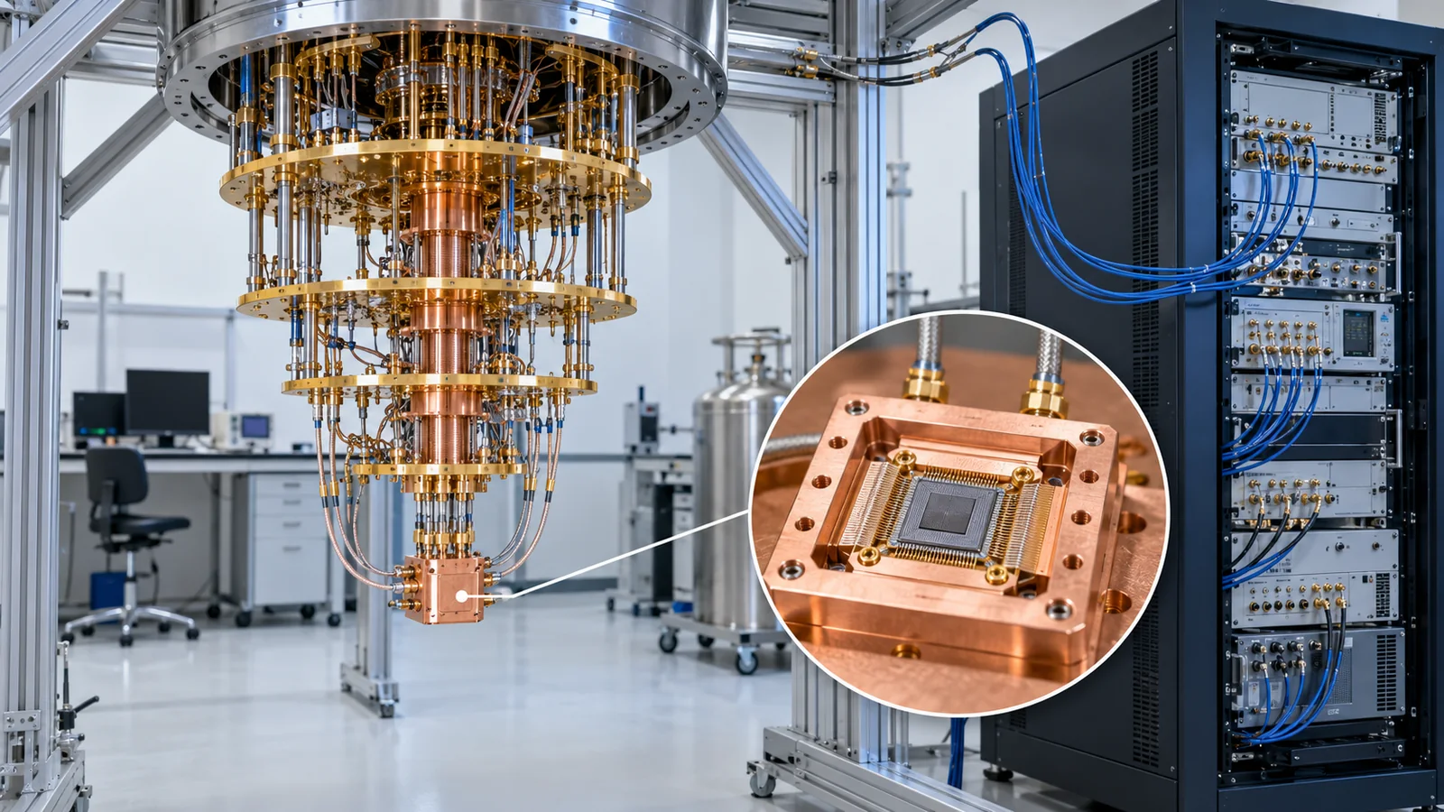
Three-line summary / what to know first / where this sits in the series
Starting point: the classical bit, and the qubit
The qubit as an "arrow"
Measurement: it fixes the answer, and there is no going back
Interference: adding waves (the heart of quantum computing)
Entanglement: two qubits acting as one unit
No-cloning: a quantum state cannot be copied
What does a quantum computer actually do? (correcting common misconceptions)
Compared with a classical computer: what it is good and bad at
How is one built? Qubit technologies and the role of materials
Where things stand (checked 16 October 2026)
How to read evaluations and standards
Glossary
References (primary sources)
Claim-to-source audit

Notation used in this article

Sourced = stated in a published source (link given)
Our calculation = a value this article computed from stated assumptions
Not yet confirmed = company targets and plans, standards still being drafted, and other items that are not settled
Our own reading for materials engineers is marked as commentary; inference is shown in bold. Every analogy comes with a note on where the analogy breaks down.

How to read the numbers in this article

The probabilities, amplitudes and state counts in Chapters 3 to 6 are our own illustrative calculations (with fixed random seeds), not measurements from a real device. Performance claims and plans from companies are reported as that company's claims; we do not rank them. For standards (ISO/IEC, IEEE) we confirmed only the title, scope and status, not the text. This field moves fast, so equipment, plans and standards carry a check date (16 October 2026).

1. Three-line summary / what to know first / where this sits in the series

A qubit is an "arrow": a classical bit is either 0 or 1; a qubit can be drawn as an arrow from the centre of a sphere. North is 0, south is 1, and a tilted arrow is a "superposition". But when you measure it, you get 0 or 1, and the original arrow does not come back Sourced [Ref. 1]
The weapon is "interference": quantum states can be added like waves. By building a computation in which the waves of the right answer reinforce and those of wrong answers cancel, some problems become faster to solve. It does not compute all answers at once and pick the best Sourced [Refs. 9, 11]
It is not a universal speed-up machine: only a limited set of problems are known to speed up, and most everyday tasks (spreadsheets, documents, video) gain nothing. The hardware is also still fighting noise (errors) Sourced [Refs. 2, 11, 22]

What to know before reading

You need no background. A picture of a bit (0 or 1) and of waves (ripples on water that add together) is enough. Formulas are kept to a minimum; when one appears, we explain it in words and check it with a number. Harder material is tucked into folded "More detail" sections.

Where this sits in the series

This is the first article to read in the Quantum Computing series. Next come "Quantum Gates and Quantum Circuits" (how arrows are rotated), then "Coherence and Fidelity" (the yardsticks for hardware quality) and "Quantum Algorithms" (why it can be faster). Technology-specific articles (superconducting, ion, neutral atom and so on), error correction, cryptography and chemistry applications are covered in their own articles in the series.

2. Starting point: the classical bit, and the qubit

Let us first recall the unit of information in everyday computers. In a smartphone or PC, information is stored in bits. A bit is either "0" or "1", corresponding, say, to no current or current flowing. You can see its value, it does not change when you look, and you can copy it as many times as you like.

A qubit (quantum bit) also has two states called "0" and "1", but it is not limited to them. It can take infinitely many states in between. The next figure shows the difference.

Fig. 2 Conceptual diagram (vector drawing). Left: a classical bit (0 or 1). Right: a qubit (an arrow in a sphere). We use this arrow picture throughout the series. The drawing is explanatory, not the structure of any real device.

A stumbling block: "a qubit is 0 and 1 at the same time"

You may have heard this. It is a common way of putting it, but this article does not use it, because it leads to misunderstandings (see the "common misconceptions" in Chapter 8). Instead, think "the arrow points somewhere". An arrow pointing north is "0", pointing south is "1", and a tilted arrow shows how much of each is "mixed in". That is what is called a "superposition".

3. The qubit as an "arrow"

The state of a single qubit can be drawn as an arrow from the centre of a sphere to its surface. The sphere is called the Bloch sphere. We fix the north pole as "0" and the south pole as "1". This is the standard picture in textbooks [Ref. 1] and in IBM Quantum Learning [Ref. 35] Sourced.

Fig. 3 Conceptual diagram (vector drawing). The arrow picture of a qubit (the Bloch sphere). θ is the angle between the arrow and the north pole. The picture works only for a single qubit; once several qubits are entangled it no longer applies (Chapter 6).

(1) The tilt of the arrow sets how likely each result is

What happens if you "measure" a tilted arrow? The result is either 0 or 1, but which one comes out is a probability set by the tilt. The closer to north, the likelier a 0; right on the equator, it is 50:50. If the tilt angle is θ (0° for due north, 180° for due south), the probability of getting 0 is cos²(θ/2) Sourced [Ref. 1].

Fig. 4 Chart including our calculation (vector drawing). Relation between tilt θ and the measurement probabilities (P(0) = cos²(θ/2)). The curve is our own calculation, not data from any real device. The relation is the standard one found in textbooks [Ref. 1].

Tilt θ	Arrow direction	Probability of "0"	Probability of "1"
0°	due north	100%	0%
60°	tilted towards north	75%	25%
90°	on the equator	50%	50%
120°	tilted towards south	25%	75%
180°	due south	0%	100%

Our calculation. We evaluated cos²(θ/2) at θ = 0°, 60°, 90°, 120° and 180° (at 30° it is 93.3% : 6.7%). As a check, at 60° cos²(30°) = 0.75.

(2) The arrow's other piece of information: its heading (phase)

Besides its tilt from north, the arrow has a second piece of information: which way it points around the north-south axis (like longitude on Earth). This is called the phase. Measuring directly does not show it in the 0/1 probabilities. But as Chapter 5 shows, it is vital information when waves are added together (interference), because it changes the result.

More detail: in formulas (safe to skip)

The state of a qubit is written α|0⟩ + β|1⟩ using two numbers α and β (complex numbers called amplitudes). The probability of "0" is |α|², that of "1" is |β|², and they add up to 1. With the arrow's tilt θ and heading φ, α = cos(θ/2) and β = e^iφ sin(θ/2) [Ref. 1]. The probability table above follows from this: at θ = 60°, α = cos 30° ≈ 0.866 and |α|² = 0.75 (Our calculation). A symbol such as |0⟩ simply means "the state 0"; in this article it is used only to label figures.

Where the analogy breaks down: the arrow picture works only for a single qubit

The arrow describes one qubit exactly. Once two or more qubits become "entangled" (Chapter 6), you can no longer draw one arrow for each. And the arrow only shows what the state looks like; it does not explain why (our commentary).

4. Measurement: it fixes the answer, and there is no going back

Reading out a qubit is called measurement. It has three properties that a classical bit does not Sourced [Ref. 1].

The result is 0 or 1, never in between: even for a tilted arrow, what comes out is "0" or "1" (never something like "0.3")
After measurement, the arrow points the way of the result: if "0" comes out it points north, if "1" south; the original tilted arrow does not come back
One measurement does not reveal the original tilt: a single measurement gives just one 0 or 1. To learn the tilt you repeat the same preparation many times and count how often 0 and 1 appear

Fig. 5 Chart including our calculation (vector drawing). One measurement yields a single 0 or 1, so the same circuit is run many times to estimate the probabilities. The bars come from our own simulation (1000 shots, random seed 0), not from a real device.

For example, prepare an arrow tilted by 60° a thousand times and measure each. In theory "0" appears about 750 times and "1" about 250 times. In our simulation (seed 0), 0 appeared 733 times and 1 appeared 267 times Our calculation. Each single result is as unpredictable as a die roll, but with more repetitions the ratio approaches the theoretical value.

A stumbling block: measuring is not "peeking inside"; it changes the state

Looking at a classical bit does not damage it. For a qubit, the act of measuring itself changes the state. Think of it not as "looking at a glass bead" but as "touching a glass bead and judging by feel whether it is north or south". After you touch it, the bead is no longer as it was. Where the analogy breaks down: real measurement is a physical interaction between an instrument and the qubit; nothing is literally "touched".

More detail: measuring n qubits gives only n bits

As we will see, writing down the state of n qubits can take 2ⁿ numbers (amplitudes). Yet what you can extract by measuring is just one string of n zeros and ones. The textbook [Ref. 1] treats the result (Holevo's theorem) that n qubits can deliver at most n bits of classical information (our commentary). This is one reason a quantum computer does not "compute every answer at once" (Chapter 8).

5. Interference: adding waves (the heart of quantum computing)

(1) First, an everyday kind of wave

When two ripples meet on water, the water rises where crest meets crest and stays calm where crest meets trough. This is interference. The first case is called reinforcement and the second cancellation.

Fig. 6 Conceptual diagram (vector drawing). Conceptual diagram of interference. Waves of the same shape reinforce when overlaid and cancel when crest meets trough. The wave shapes are drawn for explanation.

(2) The "waves" of a qubit: amplitudes

In the quantum world, the numbers from which the probabilities of measuring 0 or 1 are built behave like waves. These numbers are the amplitudes (wave heights) from Chapter 3. Two points matter Sourced [Ref. 1]:

Amplitudes can be positive or negative. Probabilities cannot be negative, but amplitudes can, so adding them can cancel
The probability of measuring "0" is the amplitude arriving at "0" added up first, then squared (not squared first and then added)

(3) Try it: applying the same operation twice

Let us use one operation specific to qubits. It tips a north-pointing (0) arrow down to the equator, giving a 50:50 state. It is called the H (Hadamard) gate (see "Quantum Gates and Quantum Circuits"). What happens if we apply this "make it 50:50" operation twice in a row?

With a coin, tossing twice still gives 50:50. But the qubit returns to north. The reason is interference. Follow the "paths" in the next figure.

Fig. 7 Chart including our calculation (vector drawing). On a qubit, applying the same operation (H) twice makes the two paths reinforce at |0⟩ and cancel at |1⟩. 0.71 approximates 1/√2; the amplitude arithmetic is our own calculation, checked numerically.

Final state	Amplitudes of the two arriving paths	Sum	Probability when measured (sum squared)
"0"	0.71×0.71 and 0.71×0.71 (both positive)	0.5 + 0.5 = 1	100% (reinforcement)
"1"	0.71×0.71 and 0.71×(−0.71) (one negative)	0.5 − 0.5 = 0	0% (cancellation)

Our calculation. 0.71 approximates 1/√2 ≈ 0.7071. We applied H twice by matrix multiplication and confirmed numerically that the result is (1, 0), that is, back to north. The definition of H follows the textbook [Ref. 1].

A stumbling block: a "random 0 or 1" is not the same as a "superposition"

A 50:50 state looks like a coin toss: measure once and you get a random 0 or 1. The difference shows up when you operate again without measuring. A coin (probabilities only) can only add; a qubit (amplitudes) can also subtract (cancel). This cancellation is why a quantum computer has a power that a classical probabilistic computer lacks (our commentary; theory in Refs. 9, 11).

A materials engineer's view 1: interference is very fragile against a disturbed environment

Interference works only when the phases (timing) of the waves line up. If the timing slips even slightly, cancellation becomes incomplete and a "1" appears where none should. A qubit's phase is disturbed by fluctuations in magnetic and electric fields and by defects in the materials around it. This is "decoherence", covered in "Coherence and Fidelity". For a materials engineer the lesson is that a qubit's performance is set by the purity of the materials and the quality of the interfaces (concrete examples in Chapter 10; our commentary).

6. Entanglement: two qubits acting as one unit

(1) Treating two qubits as a single whole

With two qubits, you can normally draw "arrow A" and "arrow B" separately. But if you apply a special operation to the pair (the CNOT gate, covered in "Quantum Gates and Quantum Circuits"), you can end up in a state where neither qubit alone has a state you can write down. This is entanglement.

A typical example is a state where the combinations "00" and "11" are overlaid as waves of equal height (a Bell state). If you measure both qubits of this pair, the result is either "00" or "11"; "01" and "10" never appear. Which one you get is random every time Sourced [Ref. 1].

Fig. 8 Chart including our calculation (vector drawing). The idea of entanglement. Measuring both qubits gives matching results every time, yet either one alone looks like a random 0 or 1. The 12-run sample and the 1000-run tally come from our own simulation (random seed 1).

(2) The "pair of gloves" analogy, and its limit

Here is a familiar analogy. Put a right-hand glove and a left-hand glove in separate boxes and send them far apart. If you open one box and find the right glove, you know the other holds the left. This is a classical correlation: the contents were fixed before anyone opened a box.

Experiments have shown that entanglement cannot be explained this way. If the idea that "results are fixed before measurement" (local hidden-variable theory) were right, a certain inequality (a Bell inequality) would hold. Experiments have shown it being violated. Hensen and colleagues reported a violation with electron spins 1.3 km apart, closing the detection loopholes at the same time Sourced [Ref. 7]. The 2022 Nobel Prize in Physics was awarded to Aspect, Clauser and Zeilinger "for experiments with entangled photons, establishing the violation of Bell inequalities and pioneering quantum information science" Sourced [Ref. 8].

Where the analogy breaks down: gloves are fixed before the box is opened, which entangled qubits are not. The glove analogy also cannot explain the correlations you get when you change how you measure (for example, east-west instead of north-south) (our commentary).

Common misconception: "entanglement sends information instantly" is wrong

Seen alone, the result at A is a random 0 or 1. Someone at B cannot tell, from B's data alone, what A measured or even whether A measured at all. Only when the two people compare their results does the perfect match appear. Comparing needs an ordinary channel (no faster than light). So entanglement alone cannot carry a message (our commentary; how entanglement is used in communication is covered in our article on quantum networks and repeaters).

(3) Entanglement makes the number of states explode

For one qubit, you need two numbers (amplitudes) to write the state. For two qubits, four; for three, eight. Each extra qubit doubles the count. For entangled qubits, writing the state of n qubits generally takes 2ⁿ numbers Sourced [Refs. 1, 4] (without entanglement, 2n numbers are enough).

Fig. 9 Chart including our calculation (vector drawing). The count of numbers (2ⁿ complex amplitudes) and memory needed to write an n-qubit state directly on a classical computer. It is our own calculation using 16-byte double-precision complex numbers, not a specification of any machine. Bar lengths are only indicative (the true ratios are vastly larger).

For example, writing the state of 50 qubits straight into a classical computer's memory, at 16 bytes (a double-precision complex number) per amplitude, takes about 16 PiB (2⁵⁰ × 16 bytes) Our calculation. In 1982 Feynman pointed out that following a quantum system on a classical computer becomes very costly as the system grows, and proposed simulating quantum systems with quantum parts instead Sourced [Ref. 4]. This is one of the starting points of quantum computing.

A stumbling block: "2ⁿ states" is not "2ⁿ answers"

Being able to hold 2ⁿ amplitudes is not the same as being able to read out 2ⁿ results. As Chapter 4 showed, measurement returns just one string of n zeros and ones. Picture "owning a huge table, but you can look at only one cell at a time, and looking destroys the table". That is why you must shape the contents of the table by interference so that the answer you want is the likely one (Chapter 8).

7. No-cloning: a quantum state cannot be copied

Classical information can be copied any number of times: read it and write the same thing. Quantum states are different. In 1982 Wootters and Zurek, and Dieks, showed that no device can make an exact copy of an unknown quantum state (the no-cloning theorem) Sourced [Refs. 5, 6].

Fig. 10 Conceptual diagram (vector drawing). Copying classical information versus a quantum state. That an unknown quantum state cannot be cloned was shown in 1982 by Wootters and Zurek, and by Dieks [Refs. 5, 6].

The intuition comes from the measurement in Chapter 4. To copy something, you first have to "read" it. But reading (measuring) changes the state and collapses the tilt of a tilted arrow into 0 or 1 (our commentary).

Why this matters

Error correction has to work differently: classical communication can fix errors by "keeping three copies and taking a majority vote". Quantum states cannot do this. Instead, information is spread over many physical qubits (using entanglement) so that one "logical qubit" is protected redundantly (see our article on quantum error correction and the surface code)
Eavesdropping-resistant communication becomes possible: in quantum key distribution (QKD), the fact that an eavesdropper cannot perfectly copy the quantum states on the line is explained as one basis of its security Sourced [Ref. 33] (see our article on QKD and quantum communication)

A stumbling block: a state known to be 0 or 1 can be copied

What cannot be copied is a state you do not know (a tilted arrow, for example). A state known to be "north or south" can be copied onto another qubit with a CNOT gate. But if you apply the same "copy" to a tilted arrow, you do not get a copy; you get entanglement (see "Quantum Gates and Quantum Circuits").

8. What does a quantum computer actually do? (correcting common misconceptions)

Combine the parts so far (arrows, measurement, interference, entanglement) and a quantum computation can be described in three steps.

Fig. 11 Conceptual diagram (vector drawing). Conceptual diagram of the three stages of a quantum computation. Bar heights are illustrative, not the values of a specific algorithm; it shows the design idea of using interference to boost the answer.

Prepare: set the qubits to the initial state (north) and, with an operation, give many candidates waves of equal height
Design the interference: line up operations (quantum gates) that add and subtract the waves, so that the waves of the right answer reinforce and the waves of wrong answers cancel
Measure: at the end, measure. Candidates with taller waves are likelier, so the right answer comes out with high probability. If one run is not enough, repeat and take a majority vote

Boiled down, designing a quantum algorithm means "designing waves so that the right answer reinforces" Sourced [Ref. 11]. Specific algorithms are covered in "Quantum Algorithms".

Common misconception 1: "a quantum computer computes all answers at once and picks the best" is wrong

This explanation is widespread but not accurate, for two reasons. (1) Even if many candidates are "in" the state, measurement extracts only one, chosen by probability (Chapters 4 and 6). (2) Without some design, what you measure is just one random candidate. To get the right answer with high probability you need interference that boosts it.

In fact, for "unstructured search where you are only given a function that checks whether a candidate is right", Bennett and colleagues showed that a quantum computer can cut the number of tries only to about the square root of brute force Sourced [Ref. 9]. If it could "compute everything at once and select", such a limit would not appear.

Common misconception 2: "more qubits means higher performance" is wrong

The number of qubits is only part of performance. If errors are frequent, a long computation breaks midway however many qubits there are. Also, physical qubits (the actual parts) and logical qubits (high-quality qubits protected by error correction and usable for computation) are counted in entirely different ways. When you hear "how many qubits", always ask physical or logical, what the error rate is, and how many operations can be run in a row (Chapter 12).

9. Compared with a classical computer: what it is good and bad at

Item	Classical computer	Quantum computer
Unit of information	bit (0 or 1)	qubit (direction of an arrow); measuring gives 0 or 1
How the state is written	n bits are a string of n zeros and ones	n qubits generally need 2ⁿ amplitudes (when entangled)
Basic operation	logic gates (AND, NOT and so on)	quantum gates (rotate the arrow; reversible)
How computation proceeds	follows a fixed procedure to a result	raises the probability of the right answer by interference
Reading out the result	can be read any number of times	measuring destroys the state; repeat and estimate probabilities
Copying	free	impossible for unknown states (no-cloning)
Resistance to errors	very strong (extremely low error rate)	weak; noise disturbs the state; error correction is essential
Good at	almost all everyday computation	a limited set of problems (factoring, simulating quantum systems and so on)

This summary is our commentary (basis: Refs. 1, 2, 5, 9, 11). The remark on classical error rates is a general statement, not tied to a specific source value.

Fig. 12 Conceptual diagram (vector drawing). A sorting of problems where quantum computers are expected to help and where they are not (conceptual). These are theoretical outlooks, not speed-ups confirmed on real machines.

Even for the "green" problems, "faster" holds in theory, with a sufficiently large error-corrected machine. Montanaro's survey organises quantum algorithms by the size of the speed-up (exponential, quadratic and so on) Sourced [Ref. 11]. Babbush and colleagues estimate that a quadratic speed-up is likely not to pay off on early error-corrected machines, because of the heavy overhead of error correction Sourced [Ref. 12]. For ground-state energies in quantum chemistry, one assessment concludes that evidence for an exponential speed-up across chemistry has not yet been found Sourced [Ref. 13].

A stumbling block: a quantum computer is not the "next generation" of the PC

Quantum computers are usually described not as a replacement for classical computers but as a different kind of machine for solving particular problems faster. Most schemes use them together with classical computers (for preparation and post-processing) (our commentary; see our article on NISQ and hybrid computing). There is generally no point in running spreadsheets or the web on a quantum computer.

10. How is one built? Qubit technologies and the role of materials

(1) What a qubit needs (DiVincenzo's five criteria)

What does it take to build a quantum computer? In a 2000 paper, DiVincenzo of IBM set out five requirements, plus two more for carrying quantum information between places Sourced [Ref. 3]. The table restates the five in this article's plain words (the restatement is our commentary).

Requirement (DiVincenzo)	Plain restatement	Link to earlier chapters
1. A scalable physical system with well-characterised qubits	You can line up many qubits of the same quality	Chapter 9. Increasing the number while keeping the quality is the challenge
2. The ability to initialise the state	Before computing, you can set everything to "north (0)"	"Prepare" in Chapter 4
3. Coherence times much longer than the gate operation time	You can do many operations before the arrow blurs	Interference in Chapter 5; "Coherence and Fidelity"
4. A universal set of quantum gates	You can rotate the arrow to any direction you need	"Quantum Gates and Quantum Circuits"
5. Qubit-specific measurement capability	You can read out 0 or 1 one qubit at a time	Measurement in Chapter 4

The content of the five requirements follows DiVincenzo (2000) [Ref. 3] Sourced. The mapping in the right-hand column is our commentary.

(2) "What to make a qubit from" is still not settled

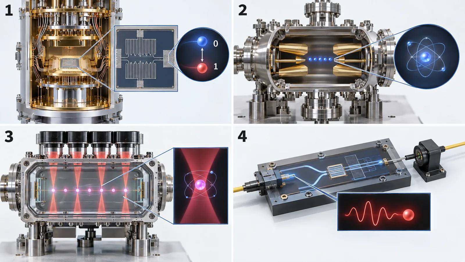
Anything physical that can carry the "direction" of an arrow can serve as a qubit. At present these main technologies are being researched and developed. Strengths, weaknesses and numbers for each are covered in the series' dedicated articles.

**Fig. 13. Conceptual illustration generated with ImageGen.** 1: superconducting circuit; 2: ions above electrodes; 3: neutral atoms in optical tweezers; 4: photonic components. Particle symbols are enlarged schematic representations, not naked-eye views. Not an actual product, facility, dimensional specification or measurement. Distinguish enlarged models from full-scale scenes.

View original SVG, values and sources

Original SVG reference: Conceptual diagram (vector drawing). Examples of the main qubit technologies. A conceptual diagram based on DiVincenzo's framework [Ref. 3] and review articles [Refs. 15-20]; not the structure of any real device.

Superconducting circuits: small electrical circuits made of a metal that loses electrical resistance at very low temperatures. Reviews describe using two energy states of a circuit as the qubit and operating it in a dilution refrigerator at about 10 mK (millikelvin, close to absolute zero) Sourced [Ref. 15]. The 2025 Nobel Prize in Physics went to Clarke, Devoret and Martinis "for the discovery of macroscopic quantum mechanical tunnelling and energy quantisation in an electric circuit" Sourced [Ref. 30] (the link to superconducting qubits is our commentary)
Trapped ions: internal states of ions held in vacuum by electromagnetic fields [Ref. 16]
Neutral atoms: atoms held one by one by laser light and arranged in arrays [Ref. 17]
Photons: the path or polarization of particles of light [Ref. 18]
Spins in silicon and other semiconductors: the spin of an electron in a semiconductor [Ref. 19]
Topological: a research-stage approach [Ref. 20]

Caution: which technology will become mainstream has not been settled

The technologies differ greatly in operation speed, error rate, ease of scaling and the environment they need (temperature, vacuum), and strengths and weaknesses trade places. Do not rank a number from one technology against a number from another; the conditions differ. A company's announcement describes results in that company's own technology, as that company's claim (our commentary).

**Fig. 14. Conceptual illustration generated with ImageGen.** A scene of making and inspecting a qubit chip. Qubit performance depends on the quality of materials and interfaces (materials engineer's views 2 and 3). It does not depict any real facility or product. Not an actual product, facility, dimensional specification or measurement. Distinguish enlarged models from full-scale scenes.

(3) A materials engineer's view: a qubit is only as good as its materials

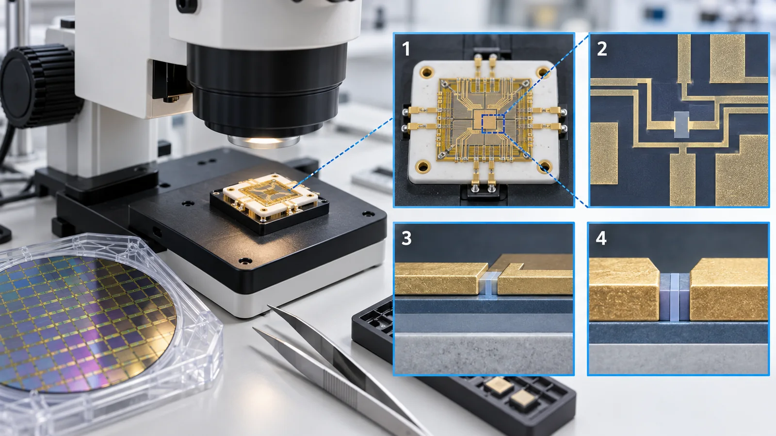
A materials engineer's view 2: what shortens a qubit's lifetime is surfaces, interfaces and contamination

A superconducting qubit consists of a metal thin film, a substrate and an extremely thin insulating film (the Josephson junction). The literature points to surfaces, interfaces and contaminants in the materials as causes of a shortened lifetime (the time before it loses energy). Place and colleagues reported that replacing niobium with tantalum raised both the lifetime and the coherence time (with dynamical decoupling) of two-dimensional transmon qubits above 0.3 ms, and that lifetimes improved in seventeen devices Sourced [Ref. 31].

Bland and colleagues then reported that changing the substrate under the tantalum film to high-resistivity silicon sharply reduced the substrate loss and gave a best lifetime (T₁) of up to 1.68 ms (the average quality factor over 45 qubits was 9.7×10⁶). In earlier tantalum-on-sapphire devices the loss was dominated by microscopic defects called two-level systems (TLS), with surface and substrate contributing about equally Sourced [Ref. 38]. A review of TLS is given by Müller and colleagues [Ref. 34]. These are laboratory results, not the performance of mass-produced machines. For a materials engineer: "which metal", "which substrate" and "how the interface is made" translate directly into qubit performance (our commentary; a review of the materials challenges is given by de Leon and colleagues [Ref. 21]).

A materials engineer's view 3: a "quiet crystal" with controlled isotopes lengthens a qubit's life

In silicon spin qubits, the magnetism of atomic nuclei in the crystal is one source of disturbance. Natural silicon contains ²⁹Si, which carries a nuclear spin. Muhonen and colleagues reported that in a nanostructure built on a substrate enriched in ²⁸Si, which has no nuclear spin, the nuclear-spin qubit of a ³¹P atom showed a coherence time over 30 s with a CPMG sequence, with control fidelity above 99.99% Sourced [Ref. 39]. It is an example of controlling even the isotopes of a material bringing a direct gain in qubit lifetime (a review of isotope engineering is given by Itoh and Watanabe [Ref. 32]; our commentary).

A materials engineer's view 4: materials and processes that "support" qubits are also covered in earlier articles of this series

Besides the qubits themselves, a quantum computer rests on many materials and processes: cryogenic wiring, refrigerators, read-out amplifiers, lasers, optical fibre and detectors. The series already covers related building blocks in these articles: quantum dots, atomic layer deposition (building thin insulating films one atomic layer at a time), nanometrology, spintronic materials, thin-film lithium niobate, silicon nitride waveguides, silicon photonics, photodetectors, semiconductor lasers and optical fiber. Our article on materials and fabrication for quantum computers organises them from the quantum-computer point of view.

11. Where things stand (checked 16 October 2026)

This field changes quickly, so here we summarise what we could confirm from primary sources, with a check date. Company claims are reported as that company's claims.

Item	What we could confirm	Category
A way to describe the present stage	In 2018 Preskill proposed the era of noisy intermediate-scale quantum (NISQ) devices. He wrote that devices with 50 to 100 qubits may be able to perform tasks that surpass classical computers, but that noise in quantum gates will limit the size of circuits that can be run reliably [Ref. 2]	Sourced
"Quantum advantage" claims	In 2019 a Google team reported that its 53-qubit superconducting processor Sycamore sampled a random circuit in about 200 seconds, a task it estimated would take a state-of-the-art supercomputer about 10,000 years (a company claim) [Ref. 14]. Pan and colleagues later reported generating samples from the same circuit with a classical tensor-network method in about 15 hours on 512 GPUs (target fidelity about 0.0037) [Ref. 36]. Read the two together and check the differences in conditions (what task, at what precision). See our article on how to read quantum-advantage claims	Sourced
Progress in error correction	Google Quantum AI reported a distance-7 surface code (101 qubits) in which the logical error rate fell by a factor of Λ = 2.14 ± 0.02 each time the code distance grew by two, with 0.143% ± 0.003% logical error per error-correction cycle. The logical memory outlived its best physical qubit by a factor of 2.4 ± 0.3 (company report) [Ref. 22]. The paper states that orders of magnitude still separate present logical error rates from what practical computation requires	Sourced
Company plan	IBM plans a fault-tolerant quantum computer, "Starling", for 2029, running 100 million quantum gates on 200 logical qubits (IBM's official page, checked 16 October 2026) [Ref. 23]	Not yet confirmed
Advantage on a practical task	Within the scope of this survey we cannot say that an advantage on a practical task over the best classical methods, including third-party verification, has been confirmed. We could not confirm it, so we do not state it	commentary

Checked 16 October 2026. Device numbers are values under each report's conditions and are not meant for ranking devices of different technologies. A roadmap is a company target and is separate from an achieved fact.

Summary of the current situation

Today's quantum computers are at the stage of "checking, on small machines, the principle of suppressing errors". Signs that error correction improves the quality of logical qubits have been reported (table above). But a "practical task done better than a classical computer" has not been confirmed. A company's plan (2029 and so on) is a target, not a guarantee.

12. How to read evaluations and standards

A quantum computer's performance cannot be captured in one number. The "number of qubits" is only a rough guide to size. You need to look together at the error rate (accuracy of operations), the coherence time (how long the arrow stays steady), the connectivity (which qubits can be operated on directly) and the accuracy of measurement. The table below sets out the methods that measure these (randomized benchmarking, quantum volume and others) and the state of the standards that fix terms and metrics, as far as we could confirm (checked 16 October 2026).

What is measured	Representative benchmark or evaluation method (name, source)	Standards and guidance (ISO/IEC, IEEE and others)	How to read it
Size in qubits	Could not be confirmed (we found no standard way to measure the number alone; physical and logical qubits are counted differently)	Terms: ISO/IEC 4879:2024 "Information technology — Quantum computing — Vocabulary" (edition 1, May 2024, IEC/ISO JTC 3) [26] Sourced / IEEE P7130 "Standard for Quantum Technologies Definitions" (on IEEE's page an active PAR, that is, a project under development; PAR approved 23 September 2021) [28] Not yet confirmed	Do not compare on the number alone; see it together with physical or logical and the error rate. We have not read the text of the standards and state none of their definitions
Accuracy of operations (gate error rate)	Randomized benchmarking (Magesan et al., 2011) [24] Sourced	Could not be confirmed (IEEE P7131 has a working group on quantum computing performance metrics and benchmarking, but we found no published standard) [37] Not yet confirmed	Check which operation, on how many qubits, and whether average or best (see "Coherence and Fidelity")
Whole-circuit performance	Quantum volume (Cross et al., 2019) [25]; application-oriented benchmarks (Lubinski et al., 2023) [27] Sourced	Could not be confirmed (as above)	No single metric expresses superiority for every use; each measures something different
Overview of benchmarking	The survey by Lorenz et al. (2025) organises benchmarks at the levels of qubits and gates, the whole processor, software and applications, and argues for standardisation [29] Sourced	Could not be confirmed	A survey's recommendations are not themselves a standard
Error-correction results	Logical error rate and the suppression factor Λ when the code distance grows (Google Quantum AI, 2024) [22] Sourced	Could not be confirmed	Check how many error-correction cycles, at what code distance. Note that it is a company report
Plans (roadmaps)	— (a plan, not an evaluation)	Could not be confirmed (there is no standard). Company target: IBM Starling (2029, 200 logical qubits) [23] Not yet confirmed	Plan and achievement are different things. Target years can change

The arrangement of this table is our own organisation (Our calculation). ISO number, title and date were checked on ISO's committee page, and the IEEE status on IEEE SA's project pages (checked 16 October 2026). Standard texts are paid or unread, so we limit ourselves to title and scope.

Reading notes (for materials engineers)

"How many qubits" alone does not tell you performance: look at error rate, coherence time, connectivity and measurement accuracy together. Physical and logical qubits are counted differently
A company's announcement and third-party verification are different: as the table in Chapter 11 shows, a company's estimate and a classical re-evaluation of the same task can sit side by side. Read both and check how the conditions differ
Check whether a standard is a recommendation or a requirement: ISO/IEC 4879 is a vocabulary, not a pass/fail performance standard. IEEE P7130 and P7131 are projects still under development. For any claim of "compliance", ask which standard and which clause
Plan and achievement are different: a roadmap (target year, target size) belongs to the unconfirmed future

13. Glossary

Bit: The unit of information in a classical computer: either "0" or "1".

Qubit (quantum bit): The unit of information in a quantum computer. It can be drawn as an arrow in a sphere; measuring gives 0 or 1.

Bloch sphere: The sphere used to draw the state of one qubit as an arrow. North pole is 0, south pole is 1.

Superposition: The arrow points neither due north nor due south but is tilted. Measuring gives 0 or 1 with probabilities set by the tilt.

Amplitude: The number from which a probability is built (a wave height). It can be positive or negative, so adding can cancel. Probability is the amplitude squared.

Phase: The arrow's heading around the north-south axis. It cannot be measured directly but changes results through interference.

Interference: Adding waves. Reinforcement raises the height; cancellation removes it. The core of quantum algorithms.

Measurement: Reading out a qubit. The result is 0 or 1, and the original state does not come back.

Entanglement: Two or more qubits form one whole, and no single one has a state of its own. It does not send information instantly.

Bell inequality: An inequality that would hold if "results are fixed before measurement" were true. Experiments have shown it violated.

No-cloning: The theorem that an unknown quantum state cannot be copied exactly.

Quantum gate: An operation that rotates a qubit's arrow. It is reversible (see "Quantum Gates and Quantum Circuits").

H (Hadamard) gate: Tips a north-pointing arrow down to the equator, creating a superposition.

CNOT: An operation on two qubits, used for example to create entanglement.

Decoherence: The environment disturbing a quantum state so that it degrades (the arrow blurs).

Physical qubit: A qubit as an actual part. It contains errors.

Logical qubit: A high-quality qubit, usable for computation, protected from errors by many physical qubits.

Quantum error correction: Protecting one logical qubit redundantly with many physical qubits. Copying is impossible, so another method is used.

NISQ: Noisy intermediate-scale quantum: the term for the era of noisy, mid-sized quantum devices (Preskill, 2018).

Quantum advantage: A claim that a quantum computer beats classical computers on some task. Who claims it, on what task, and against what comparison all matter.

Dilution refrigerator: A machine that reaches very low temperatures close to absolute zero (about 10 mK, for example). Used with superconducting qubits.

Josephson junction: Two superconductors separated by an extremely thin insulating film. The key element of a superconducting qubit.

Randomized benchmarking: A method that measures the error rate per operation using random sequences of operations.

Quantum volume: A single number for whole-device performance based on how well random circuits run (proposed by IBM).

14. References (primary sources)

Nielsen M. A., Chuang I. L. Quantum Computation and Quantum Information, Cambridge University Press (10th anniversary edition, 2010) — cambridge.org (book page)
Preskill J. "Quantum Computing in the NISQ era and beyond", Quantum 2, 79 (2018), DOI 10.22331/q-2018-08-06-79 — doi.org/10.22331/q-2018-08-06-79
DiVincenzo D. P. "The Physical Implementation of Quantum Computation", Fortschr. Phys. 48, 771–783 (2000), arXiv:quant-ph/0002077 — arxiv.org/abs/quant-ph/0002077
Feynman R. P. "Simulating physics with computers", Int. J. Theor. Phys. 21, 467–488 (1982), DOI 10.1007/BF02650179 — doi.org/10.1007/BF02650179
Wootters W. K., Zurek W. H. "A single quantum cannot be cloned", Nature 299, 802–803 (1982), DOI 10.1038/299802a0 — doi.org/10.1038/299802a0
Dieks D. "Communication by EPR devices", Phys. Lett. A 92, 271–272 (1982), DOI 10.1016/0375-9601(82)90084-6 — doi.org/10.1016/0375-9601(82)90084-6
Hensen B. et al. "Loophole-free Bell inequality violation using electron spins separated by 1.3 kilometres", Nature 526, 682–686 (2015), DOI 10.1038/nature15759 — doi.org/10.1038/nature15759
NobelPrize.org "The Nobel Prize in Physics 2022" (Aspect, Clauser, Zeilinger) — nobelprize.org/prizes/physics/2022/summary/
Bennett C. H., Bernstein E., Brassard G., Vazirani U. "Strengths and Weaknesses of Quantum Computing", SIAM J. Comput. 26, 1510–1523 (1997), DOI 10.1137/S0097539796300933 — doi.org/10.1137/S0097539796300933
Shor P. W. "Polynomial-Time Algorithms for Prime Factorization and Discrete Logarithms on a Quantum Computer", SIAM J. Comput. 26, 1484–1509 (1997), DOI 10.1137/S0097539795293172 — doi.org/10.1137/S0097539795293172
Montanaro A. "Quantum algorithms: an overview", npj Quantum Inf. 2, 15023 (2016), DOI 10.1038/npjqi.2015.23 — doi.org/10.1038/npjqi.2015.23
Babbush R. et al. "Focus beyond Quadratic Speedups for Error-Corrected Quantum Advantage", PRX Quantum 2, 010103 (2021), DOI 10.1103/PRXQuantum.2.010103 — doi.org/10.1103/PRXQuantum.2.010103
Lee S. et al. "Evaluating the evidence for exponential quantum advantage in ground-state quantum chemistry", Nat. Commun. 14, 1952 (2023), DOI 10.1038/s41467-023-37587-6 — doi.org/10.1038/s41467-023-37587-6
Arute F. et al. (Google AI Quantum) "Quantum supremacy using a programmable superconducting processor", Nature 574, 505–510 (2019), DOI 10.1038/s41586-019-1666-5 — doi.org/10.1038/s41586-019-1666-5
Krantz P. et al. "A quantum engineer's guide to superconducting qubits", Appl. Phys. Rev. 6, 021318 (2019), DOI 10.1063/1.5089550 — doi.org/10.1063/1.5089550
Bruzewicz C. D. et al. "Trapped-ion quantum computing: Progress and challenges", Appl. Phys. Rev. 6, 021314 (2019), DOI 10.1063/1.5088164 — doi.org/10.1063/1.5088164
Henriet L. et al. "Quantum computing with neutral atoms", Quantum 4, 327 (2020), DOI 10.22331/q-2020-09-21-327 — doi.org/10.22331/q-2020-09-21-327
Slussarenko S., Pryde G. J. "Photonic quantum information processing: A concise review", Appl. Phys. Rev. 6, 041303 (2019), DOI 10.1063/1.5115814 — doi.org/10.1063/1.5115814
Burkard G. et al. "Semiconductor spin qubits", Rev. Mod. Phys. 95, 025003 (2023), DOI 10.1103/RevModPhys.95.025003 — doi.org/10.1103/RevModPhys.95.025003
Nayak C. et al. "Non-Abelian anyons and topological quantum computation", Rev. Mod. Phys. 80, 1083–1159 (2008), DOI 10.1103/RevModPhys.80.1083 — doi.org/10.1103/RevModPhys.80.1083
de Leon N. P. et al. "Materials challenges and opportunities for quantum computing hardware", Science 372, eabb2823 (2021), DOI 10.1126/science.abb2823 — doi.org/10.1126/science.abb2823
Google Quantum AI "Quantum error correction below the surface code threshold", Nature 638, 920–926 (2025), DOI 10.1038/s41586-024-08449-y (arXiv:2408.13687) — doi.org/10.1038/s41586-024-08449-y
IBM "IBM Quantum technology" (plan for IBM Quantum Starling; checked 16 October 2026) — ibm.com/quantum/technology
Magesan E., Gambetta J. M., Emerson J. "Scalable and Robust Randomized Benchmarking of Quantum Processes", Phys. Rev. Lett. 106, 180504 (2011), DOI 10.1103/PhysRevLett.106.180504 — doi.org/10.1103/PhysRevLett.106.180504
Cross A. W. et al. "Validating quantum computers using randomized model circuits", Phys. Rev. A 100, 032328 (2019), DOI 10.1103/PhysRevA.100.032328 — doi.org/10.1103/PhysRevA.100.032328
ISO/IEC "ISO/IEC 4879:2024 Information technology — Quantum computing — Vocabulary" (edition 1, May 2024, IEC/ISO JTC 3; checked on ISO's committee page) — iso.org/standard/80432.html
Lubinski T. et al. "Application-Oriented Performance Benchmarks for Quantum Computing", IEEE Trans. Quantum Eng. 4, 1–32 (2023), DOI 10.1109/TQE.2023.3253761 — doi.org/10.1109/TQE.2023.3253761
IEEE SA "IEEE P7130 Draft Standard for Quantum Technologies Definitions" (project page; active PAR, PAR approved 23 September 2021; checked 16 October 2026) — standards.ieee.org/ieee/7130/10680/
Lorenz J. M. et al. "Systematic benchmarking of quantum computers: status and recommendations", arXiv:2503.04905 (2025) — arxiv.org/abs/2503.04905
NobelPrize.org "Nobel Prize in Physics 2025" (Clarke, Devoret, Martinis) — nobelprize.org/prizes/physics/2025/summary/
Place A. P. M. et al. "New material platform for superconducting transmon qubits with coherence times exceeding 0.3 milliseconds", Nat. Commun. 12, 1779 (2021), DOI 10.1038/s41467-021-22030-5 — doi.org/10.1038/s41467-021-22030-5
Itoh K. M., Watanabe H. "Isotope engineering of silicon and diamond for quantum computing and sensing applications", MRS Commun. 4, 143–157 (2014), DOI 10.1557/mrc.2014.32 — doi.org/10.1557/mrc.2014.32
Gisin N. et al. "Quantum cryptography", Rev. Mod. Phys. 74, 145–195 (2002), DOI 10.1103/RevModPhys.74.145 — doi.org/10.1103/RevModPhys.74.145
Müller C., Cole J. H., Lisenfeld J. "Towards understanding two-level-systems in amorphous solids: insights from quantum circuits", Rep. Prog. Phys. 82, 124501 (2019), DOI 10.1088/1361-6633/ab3a7e — doi.org/10.1088/1361-6633/ab3a7e
IBM Quantum Learning "Basics of quantum information" (introductory course; consulted for the arrow and Bloch-sphere picture) — quantum.cloud.ibm.com/learning/en/courses/basics-of-quantum-information
Pan F., Chen K., Zhang P. "Solving the Sampling Problem of the Sycamore Quantum Circuits", Phys. Rev. Lett. 129, 090502 (2022), DOI 10.1103/PhysRevLett.129.090502 — doi.org/10.1103/PhysRevLett.129.090502
IEEE SA "Quantum Benchmarking Working Group P7131" (page of the working group on standardising quantum computing performance metrics; checked 16 October 2026) — sagroups.ieee.org/7131
Bland M. P. et al. "Millisecond lifetimes and coherence times in 2D transmon qubits", Nature 647, 343–348 (2025), DOI 10.1038/s41586-025-09687-4 — doi.org/10.1038/s41586-025-09687-4
Muhonen J. T. et al. "Storing quantum information for 30 seconds in a nanoelectronic device", Nat. Nanotechnol. 9, 986–991 (2014), DOI 10.1038/nnano.2014.211 — doi.org/10.1038/nnano.2014.211

15. Claim-to-source audit

Claim in the text	Basis	Category
A qubit state is drawn as an arrow on the Bloch sphere; for tilt θ the probability of "0" is cos²(θ/2); measurement gives 0 or 1 and changes the state; the H gate and so on	Textbook (Nielsen and Chuang); IBM Quantum Learning Reference 1 https://www.cambridge.org/highereducation/books/quantum-computation-and-quantum-information/01E10196D0A682A6AEFFEA52D53BE9AE Reference 35 https://quantum.cloud.ibm.com/learning/en/courses/basics-of-quantum-information	Sourced
The NISQ framing (possibility for 50 to 100 qubits, and the limit that gate noise places on circuit size)	Abstract of Preskill (2018) Reference 2 https://doi.org/10.22331/q-2018-08-06-79	Sourced
DiVincenzo's five requirements (and two for communication)	Abstract of DiVincenzo (2000) Reference 3 https://arxiv.org/abs/quant-ph/0002077	Sourced
The difficulty of following quantum systems on classical computers, and Feynman's idea of simulating them with quantum parts	Title and bibliographic data of Feynman (1982) Reference 4 https://doi.org/10.1007/BF02650179	Sourced
An unknown quantum state cannot be cloned (1982)	Titles and bibliographic data of Wootters and Zurek, and of Dieks Reference 5 https://doi.org/10.1038/299802a0 Reference 6 https://doi.org/10.1016/0375-9601(82)90084-6	Sourced
A reported Bell-inequality violation with electron spins 1.3 km apart; the stated reason for the 2022 Nobel Prize in Physics	Title and bibliographic data of Hensen et al. (2015); NobelPrize.org Reference 7 https://doi.org/10.1038/nature15759 Reference 8 https://www.nobelprize.org/prizes/physics/2022/summary/	Sourced
For unstructured search a quantum computer cuts the tries only to about the square root of brute force (relative to an oracle); the question of whether all of NP can be solved in quantum polynomial time	Abstract of Bennett et al. (1997) Reference 9 https://doi.org/10.1137/S0097539796300933	Sourced
Shor's result that factoring is solvable in polynomial time on a quantum computer; a survey organising quantum algorithms by size of speed-up	Title of Shor (1997); survey by Montanaro (2016) Reference 10 https://doi.org/10.1137/S0097539795293172 Reference 11 https://doi.org/10.1038/npjqi.2015.23	Sourced
Quadratic speed-ups are likely not to pay off on early error-corrected machines; the assessment that evidence for an exponential speed-up in ground-state quantum chemistry has not yet been found	Abstracts of Babbush et al. (2021) and Lee et al. (2023) Reference 12 https://doi.org/10.1103/PRXQuantum.2.010103 Reference 13 https://doi.org/10.1038/s41467-023-37587-6	Sourced
Sycamore (53 qubits) about 200 seconds versus an estimated 10,000 years for a classical supercomputer (company claim); samples of the same circuit generated classically on 512 GPUs in about 15 hours	Arute et al. (2019); Pan et al. (2022) Reference 14 https://doi.org/10.1038/s41586-019-1666-5 Reference 36 https://doi.org/10.1103/PhysRevLett.129.090502	Sourced
Overviews of superconducting, ion, neutral-atom, photonic, silicon-spin and topological approaches; superconducting circuits operated in an environment of about 10 mK	Review articles for each approach Reference 15 https://doi.org/10.1063/1.5089550 Reference 16 https://doi.org/10.1063/1.5088164 Reference 17 https://doi.org/10.22331/q-2020-09-21-327 Reference 18 https://doi.org/10.1063/1.5115814 Reference 19 https://doi.org/10.1103/RevModPhys.95.025003 Reference 20 https://doi.org/10.1103/RevModPhys.80.1083	Sourced
The stated reason for the 2025 Nobel Prize in Physics (macroscopic quantum mechanical tunnelling and energy quantisation in an electric circuit)	NobelPrize.org Reference 30 https://www.nobelprize.org/prizes/physics/2025/summary/	Sourced
Replacing niobium with tantalum raised lifetime and coherence time above 0.3 ms (17 devices); a high-resistivity silicon substrate gave a lifetime up to 1.68 ms and 99.994% single-qubit gate fidelity; loss dominated by two-level systems (TLS)	Abstracts of Place et al. (2021) and Bland et al. (2025) Reference 31 https://doi.org/10.1038/s41467-021-22030-5 Reference 38 https://doi.org/10.1038/s41586-025-09687-4	Sourced
On a ²⁸Si substrate a ³¹P nuclear spin kept coherence over 30 s (CPMG) with control fidelity above 99.99%; reviews on isotope engineering, TLS and materials challenges	Abstract of Muhonen et al. (2014); titles and bibliographic data of the reviews Reference 39 https://doi.org/10.1038/nnano.2014.211 Reference 32 https://doi.org/10.1557/mrc.2014.32 Reference 34 https://doi.org/10.1088/1361-6633/ab3a7e Reference 21 https://doi.org/10.1126/science.abb2823	Sourced
In quantum key distribution, an eavesdropper's inability to copy quantum states perfectly is described as one basis of security	Review by Gisin et al. (2002) Reference 33 https://doi.org/10.1103/RevModPhys.74.145	Sourced
Distance-7 surface code (101 qubits), Λ = 2.14 ± 0.02, 0.143% ± 0.003% per cycle, 2.4 times the best physical qubit's lifetime; orders of magnitude still separate this from practical requirements (company report)	Paper of Google Quantum AI (arXiv 2024, published 2025) Reference 22 https://doi.org/10.1038/s41586-024-08449-y	Sourced
IBM plans Quantum Starling for 2029, with 100 million gates on 200 logical qubits (company target; checked 16 October 2026)	IBM's official page Reference 23 https://www.ibm.com/quantum/technology	Not yet confirmed
The proposals of randomized benchmarking, quantum volume and application-oriented benchmarks; a survey of benchmarking	Magesan et al. (2011), Cross et al. (2019), Lubinski et al. (2023), Lorenz et al. (2025) Reference 24 https://doi.org/10.1103/PhysRevLett.106.180504 Reference 25 https://doi.org/10.1103/PhysRevA.100.032328 Reference 27 https://doi.org/10.1109/TQE.2023.3253761 Reference 29 https://arxiv.org/abs/2503.04905	Sourced
ISO/IEC 4879:2024 "Information technology — Quantum computing — Vocabulary" (edition 1, May 2024, IEC/ISO JTC 3): number, title and publication date	ISO's committee page Reference 26 https://www.iso.org/standard/80432.html	Sourced
IEEE P7130 (Quantum Technologies Definitions) is under development (active PAR, approved 23 September 2021) and we found no published standard at the check date; the IEEE P7131 working group is active	IEEE SA pages Reference 28 https://standards.ieee.org/ieee/7130/10680/ Reference 37 https://sagroups.ieee.org/7131	Not yet confirmed
The probability table (cos²(θ/2)), the 1000-shot simulated measurement (733 and 267), the amplitude arithmetic for two H gates (0.5 + 0.5 and 0.5 − 0.5), the 12-run simulated sample, and the state-count and memory table (2ⁿ, 16 KiB to 16 PiB)	Our own calculation (Python, NumPy; fixed random seeds; 16 bytes per double-precision complex number). Not the results of any real device	Our calculation
Whether an advantage on a practical task over the best classical methods has been confirmed, including by third parties; the text of ISO/IEC 4879; the publication state of IEEE P7131; comparisons of numbers across technologies	Could not be confirmed from the primary sources available in this survey, so not stated	commentary
Readings and explanations: "interference is fragile against a disturbed environment", "measurement changes the state", the glove and glass-bead analogies and their limits, "do not rank technologies by numbers under different conditions", "a quantum computer is not a replacement"	Our own organisation and commentary based on the published material. Not views expressed by the organisations cited	commentary
That Figs. 1 to 14 are explanatory drawings and not observations of real data, and that Figs. 1 and 14 are ImageGen-generated conceptual illustrations	Note in this article	commentary

Last updated: 16 October 2026. Sources are limited to primary material (a textbook, peer-reviewed papers, and the official pages of ISO, IEEE, NobelPrize.org and the companies). Company announcements are treated as company claims, and where a third-party re-evaluation exists we show both. The numerical examples (probabilities, amplitudes, state counts, simulated measurements) are our own illustrative calculations, not results from real devices. Roadmaps are company targets, not established facts. We could not confirm the text of the standards, the publication state of IEEE P7131, or any third-party-verified advantage on a practical task, so we do not state them. All figures are explanatory conceptual diagrams or drawings that include our own calculations; Figs. 1 and 14 are ImageGen-generated conceptual illustrations.

Illustration update: 17 October 2026. References to vector drawings in the article and source tables describe the retained original SVGs. See each current caption for the foreground image format and reading guide. ImageGen illustrations are not measurements or photographs of actual products; original SVGs, values and sources remain available in expandable references.