TECHNOLOGY EXPLAINER
Quantum Annealing
Searching for the best combination as the bottom of an energy valley
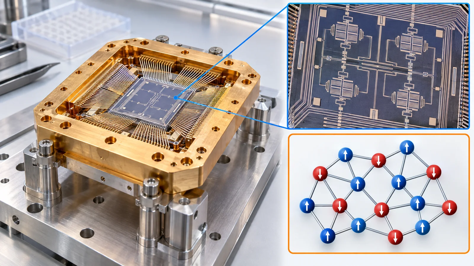
Delivery routes, shift schedules, component layouts: the world is full of problems with too many combinations to check them all. Quantum annealing rewrites such a problem as "small magnet-like spins searching for their most stable arrangement" and uses quantum effects to look for the bottom of the valley. This article first explains "combinatorial explosion" and the "Ising model" with figures, then rewrites a small numerical problem as an Ising model and runs an annealing calculation to show how it works. It then sorts out the difference from the gate model, D-Wave's approach, and the "quantum advantage" claims and the classical results that followed, keeping company claims and third-party checks apart.
- The short version, what to know first, and where this fits in the series
- Combinatorial optimization and "combinatorial explosion"
- The Ising model: the "energy" of spins that point up or down
- Mapping a problem to an Ising model: the number-partitioning example
- How quantum annealing works: weakening the sideways drive
- The minimum gap and anneal time: running a small example numerically
- How it differs from the gate model
- D-Wave's approach: a superconducting chip and its limits on connections
- Claims of "quantum advantage" and the classical results
- Limits, what we could not confirm, and a summary
- How to read evaluations and standards
- Glossary
- References
- Claim-to-source audit
Sourced = stated in a published source (linked)
Our calculation = a value computed in this article from the stated assumptions
Not yet confirmed = plans, targets, drafts, work in progress, outlooks: not settled
Our own reading for materials engineers is marked as commentary. Inference is shown in bold. Company announcements are labelled as company claims.
1. The short version, what to know first, and where this fits in the series
- Quantum annealing rewrites an optimization problem as the search for a lowest-energy state. Kadowaki and Nishimori in Japan proposed it in 1998 as simulated annealing with "quantum fluctuations" added Sourced[Ref. 1]
- The best-known device is D-Wave's superconducting chip. It works on a different principle from the gate model, so the qubit counts cannot be compared to rank them. The ISO/IEC committee for quantum computing includes quantum annealers in its scope as "restricted forms of quantum computing" Sourced[Ref. 23]
- Claims of "quantum advantage" have been followed by classical results reaching comparable accuracy. This article gives no verdict; it shows how to read claims and replies side by side Sourced[Refs. 13, 17, 18]
We use the picture of a qubit state as an arrow (north pole = 0, south pole = 1, in between = superposition) that settles on 0 or 1 when measured (see "Quantum Computing Fundamentals"). This article is readable on its own; it explains what is needed.
The maths is addition, multiplication and one energy formula. Think of "energy" as a score for a state where lower means more stable, like a ball coming to rest at the bottom of a valley.
A good order is Quantum Algorithms → NISQ and Hybrid Computing → this article. QAOA, the gate-model method with a similar aim, is in the NISQ explainer; how to read advantage claims is in the quantum advantage explainer; industrial use is in the industrial applications explainer.
2. Combinatorial optimization and "combinatorial explosion"
Combinatorial optimization means picking the best of many combinations of choices: the visiting order of delivery trucks, the sequence of jobs in a factory, combinations of material formulations. If each of n items is a yes/no choice, there are 2ⁿ combinations.
As the table in the figure shows, 30 items give about a billion combinations (about a second), 50 items about 13 days, and 100 items about 4×10¹³ years (some 3,000 times the age of the universe) Our calculation. This is combinatorial explosion. Real optimization solvers do not check everything, of course; they examine only promising parts. Even so, some problems become suddenly hard in the worst case. Lucas showed that many problems, including all of Karp's 21 NP-complete problems, can be written in Ising form Sourced[Ref. 3].
3. The Ising model: the "energy" of spins that point up or down
The common language of quantum annealing is the Ising model. There are several small magnet-like points (spins), each pointing up (+1) or down (−1). Pairs of spins have a "coupling" J: if J is positive they prefer opposite directions, and if negative they prefer the same direction. The total energy is written E = Σ hᵢsᵢ + Σ Jᵢⱼ sᵢsⱼ (h is a bias on individual spins). This form appears in D-Wave's documentation Sourced[Ref. 6].
A spin here simply means a point with a binary up/down choice (corresponding to the qubit values 0 and 1). Energy is a "badness score" for that arrangement; read lower as better. Optimization then means finding the arrangement with the lowest score (the ground state). Limit of the analogy: it is not the energy of a real magnet in units or meaning; here it is a device for expressing the problem.
4. Mapping a problem to an Ising model: the number-partitioning example
Let us rewrite a real problem as an Ising model. One of the simplest examples is the number-partitioning problem (it also appears in Lucas's paper Sourced[Ref. 3]): can a set of numbers be split into two groups with equal sums?
- Give each number aᵢ a value s = +1 (group A) or −1 (group B). Then Σ aᵢsᵢ is "the sum of group A minus the sum of group B". If it is 0, the split has equal sums.
- Taking the squared difference E = (Σ aᵢsᵢ)² as the energy makes it smallest (E = 0) when the difference is 0. Expanding gives E = Σ aᵢ² + Σi<j 2aᵢaⱼ sᵢsⱼ: a constant plus an Ising model with couplings Jᵢⱼ = 2aᵢaⱼ Our calculation
- Here the constant is Σ aᵢ² = 184 and all 15 pairs of the six spins are coupled (for example J₁₂ = 2×9×7 = 126). Evaluating all 64 splits gives two splits with E = 0 ({9,4,2} and {7,5,3}; a +/− swapped pair), and ten with E = 4 (sums differ by 2) Our calculation
(1) "0/1" and "±1" are the same thing
In optimization, variables are often written as 0/1 (QUBO: quadratic unconstrained binary optimization). The substitution s = 2x − 1 (x = 0 gives s = −1, x = 1 gives s = +1) converts between QUBO and the Ising form. Annealing devices such as D-Wave's accept either form (our commentary). The Max-Cut problem (used as the QAOA example in the NISQ explainer) is also an Ising model with J = +1 on each link (more opposite pairs means lower energy, that is, more links between different colours) Sourced[Ref. 3].
The problem must first be rewritten as an Ising model (the formulation), which is the hard part in practice. "Following the rules" (constraints) must be added as penalty terms that raise the energy when broken, and the penalty weights strongly affect the outcome (our commentary; Lucas's paper catalogues formulations of many problems Sourced[Ref. 3]). The right reading: what quantum annealing solves is "finding the lowest energy of an Ising model"; whether the real problem can be mapped onto it correctly decides half the outcome.
5. How quantum annealing works: weakening the sideways drive
How, then, do we search for the arrangement with the lowest energy? A standard method is simulated annealing. Add "heat" to shake the spins, then cool slowly, and the arrangement settles at the bottom of a valley. Thermal shaking helps the system climb over the energy hills in between.
Quantum annealing uses quantum fluctuations instead of heat. Kadowaki and Nishimori introduced a transverse field (a force that turns spins sideways), weakened over time so that it plays the role of the "temperature" in simulated annealing, and showed in numerical calculations on small systems that it reaches the ground state with higher probability than the thermal method with the same schedule Sourced[Ref. 1]. In the arrow picture it goes like this.
- Start: the sideways drive is strong and each qubit's arrow lies on the equator. A measurement gives 0 and 1 equally, so every answer is equally likely (this is a superposition, not "trying all answers").
- Midway: as the sideways drive weakens and the problem term (h and J) strengthens, each arrow gradually tilts toward the north or south pole.
- End: the problem term dominates and the arrows point nearly to a pole. Measuring gives a 0/1 string, which one hopes is an arrangement of low energy. D-Wave's documentation says A(s) ≫ B(s) at the start and A(s) ≪ B(s) at the end Sourced[Ref. 6]
The formula in D-Wave's documentation is H = −(A(s)/2) Σ σˣ + (B(s)/2) (Σ hᵢσᶻᵢ + Σ Jᵢⱼ σᶻᵢσᶻⱼ), where σˣ is the sideways drive and σᶻ the up/down direction. The anneal fraction s runs from 0 to 1 and the run time can be specified Sourced[Ref. 6]. The theoretical basis is the adiabatic theorem: if changed slowly enough, the system stays in the lowest-energy state of the moment and ends in the problem's minimum (the review by Albash and Lidar Sourced[Ref. 4]). In 2001 Farhi et al. proposed a quantum adiabatic algorithm applying this idea to random instances of an NP-complete problem Sourced[Ref. 2].
Quantum annealing is sometimes explained with "tunnelling through the hill": heat climbs over a hill whereas a quantum system slips through its thin parts. Where the analogy breaks: if the hill is tall and wide, tunnelling does not help, and whether the effect operates in a real device must be shown with separate evidence. Boixo et al. cited strong correlations between the device and a simulated quantum annealer, and weak correlations with classical annealing Sourced[Ref. 12].
It is not right to say it tries all answers at once. The initial state is a superposition in which every answer is equally likely, but a measurement settles on one answer. Think of the mechanism as designed so that the state flows into the low-energy state following the change in energy.
6. The minimum gap and anneal time: running a small example numerically
How slow is "slowly enough"? The key is the difference between the ground state (the lowest energy) and the next energy level, called the gap. If the point where the gap is smallest (the minimum gap) is not crossed slowly, the system hops to the next level and misses the answer. Roughly, the smaller the minimum gap, the longer the time needed (the typical form of the adiabatic theorem; our commentary Sourced[Ref. 4]).
Let us compute with the number-partitioning problem above (six numbers). Take H(s) = −10(1−s) Σ σˣ + s (Σ aᵢσᶻᵢ)², which starts with all arrows on the equator and ends as the partitioning energy (arbitrary units). The system has 64 states, so a laptop can compute it exactly Our calculation.
Next we ran this system through the Schrödinger equation for various anneal times T (a linear schedule s = t/T). A short T gives a low success probability, and a longer T raises it. T = 0.1 gives 8.6%, T = 1 gives 33%, T = 10 gives 80% and T = 50 gives 99.85%. A blind guess succeeds with probability 2/64 ≈ 3.1% Our calculation.
But "the longer the better" is not always true. A real device spends time on setup and readout for every run, and repeats when an answer is wrong. The "total time to a solution with 99% probability" (TTS) is estimated as TTS = (T + τ₀) × max(1, ln(1−0.99) ÷ ln(1−p)), where p is the one-run success probability. In this small example, assuming a fixed time of τ₀ = 5 per run, the total time is shortest (about 42) around T = 5 to 20, and it gets slower if T is too short or too long Our calculation. Rønnow et al. argue that to measure speedup one must compare at the best setting for each problem size Sourced[Ref. 13].
The calculation above assumes a system isolated from its environment. A real device is an "open system" affected by surrounding heat and noise, and its operating temperature is not zero. So the real device does not follow the adiabatic ideal of staying in the ground state; thermal transitions and noise also matter (our commentary). What to take from it is not the numbers but the idea of the gap, and the relation between time and success probability.
7. How it differs from the gate model
There are broadly two ways to build a "quantum computer". One is the gate model, which applies gates (operations that rotate the arrows) to the qubits one after another. The other is the annealing model, which continuously changes global strengths (A(s), B(s)). The ISO/IEC JTC 3 subcommittee on quantum computing (JSC 3A) defines its scope as universal quantum computing, restricted forms such as quantum simulators and quantum annealers, and hybrid forms Sourced[Ref. 23].
| Aspect | Gate model | Quantum annealing (D-Wave's approach) |
|---|---|---|
| Purpose | General-purpose computation (any algorithm can be written in principle) | Mainly optimization and sampling in Ising form |
| Operation | A circuit of gates run in sequence | A(s) and B(s) are changed continuously in time (the anneal) |
| How the problem goes in | Written as a quantum circuit | Entered as h and J (the Ising coefficients) |
| Qubit counts | Few, high-quality qubits (error rates, connectivity and error correction are the focus) | Thousands of qubits, but limited connectivity, and problem variables are built from chains (Fig. 9). The counts cannot be compared directly |
| Error correction | Theory and early experiments exist (other explainers) | The D-Wave material we checked contained no statement that logical-qubit error correction is performed |
| Theoretical power | Universal | General adiabatic quantum computation is polynomially equivalent to the gate model (Aharonov et al. 2007) [Ref. 5]. The power and limits of the "transverse field plus Ising" form used by D-Wave (stoquastic) are still being studied (Albash and Lidar) [Ref. 4] |
| Representative methods | Shor, Grover, VQE, QAOA and others | Quantum annealing, quantum adiabatic algorithms |
The comparison is this article's commentary; sources include [Refs. 4, 5, 23].
The two count qubits differently. Annealer qubits specialise in Ising-model optimization and have limited connections, so a large problem uses chains of several qubits for one variable (chapter 8). Gate-model qubits must carry out arbitrary gates with high accuracy. The right reading: "how many qubits" alone does not rank different approaches. Look at which task, at what accuracy, compared with what.
Incidentally, QAOA in the gate model (see the NISQ explainer) is a close relative of the quantum adiabatic idea, carried out with gates Sourced[Ref. 2].
8. D-Wave's approach: a superconducting chip and its limits on connections
D-Wave built the first commercial quantum annealers. In 2011 Johnson et al. reported finding the ground state by quantum annealing in an artificial Ising system of eight superconducting flux qubits with programmable couplings Sourced[Ref. 9]. Boixo et al. reported evidence, from experiments on the 108-qubit D-Wave One (superconducting flux qubits), that the device performs quantum annealing Sourced[Ref. 12].
What matters in the chip design is how many partners one qubit can couple to. According to D-Wave's documentation, a qubit couples to 6 others in the Chimera topology, 15 in Pegasus and 20 in Zephyr. Pegasus is the connectivity of Advantage (each chip is fabricated with 5,640 qubits) and Zephyr that of Advantage2 Sourced[Ref. 7]. In May 2025 D-Wave announced general availability of Advantage2, citing over 4,400 qubits, Zephyr's 20-way connectivity, a 40% increase in energy scale, a 75% reduction in noise and twice the coherence Sourced[Ref. 8] (a company announcement, not figures from third-party verification).
Because connections are limited, when a problem variable couples to more partners than the chip allows, a step called minor embedding is needed. A variable is assigned to a "chain" of several qubits, tied strongly so that they act as one Sourced[Ref. 10]. The next figure is the smallest example: a triangle problem in which three variables are all linked, placed on a chip whose connections form a square.
The partitioning problem above has couplings between every pair of its six variables (15 links), so it needs chains on the chip. Cai et al. presented a practical heuristic for finding such graph minors (representing the problem graph as part of the chip graph) Sourced[Ref. 11]. The number of variables that can actually be used is smaller than the chip's qubit count (our commentary).
D-Wave's devices use superconducting flux qubits Sourced[Refs. 9, 12]. Placing thousands of qubits and tens of thousands of couplers on one chip requires stacking superconducting thin films in several layers while holding down the spread in qubit characteristics (for example variation in junction fabrication) and flux noise, because any mismatch between the programmed h and J and the device's actual values feeds straight into solution quality (our commentary).
The documentation also says a Pegasus chip is fabricated with 5,640 qubits Sourced[Ref. 7]. The number fabricated and the number usable for a problem are different, and the latter has to be checked chip by chip (our commentary). Higher connectivity (Chimera 6 → Pegasus 15 → Zephyr 20) means more wiring layers and couplers, which feeds back to materials and process as a question of fabrication difficulty and yield (see our explainer on materials and fabrication).
9. Claims of "quantum advantage" and the classical results
Quantum annealing is one of the approaches for which the question "is it faster than classical computers?" has been debated longest. The claims and results are tabulated in chronological order. A general guide to reading advantage claims is in the explainer on quantum advantage; here we focus on points specific to annealing.
| Year and study | Claim or result (as the paper states) | Reading |
|---|---|---|
| 2014 Rønnow et al. | Proposed how to define and detect speedup. On D-Wave Two (up to 503 qubits), comparing random spin-glass instances of limited precision with simulated classical and quantum annealers, they found no evidence of speedup over the whole data set and inconclusive results instance by instance. The authors note that one benchmark does not rule out speedup on other problems [Ref. 13] | The conclusion depends on which set of problems is compared |
| 2016 Denchev et al. | On a crafted problem with tall, narrow energy barriers (945 variables), D-Wave 2X was about 10⁸ times faster than simulated annealing on a single core (time to 99% success). The authors note, however, that some classical heuristics solve such instances in comparable time [Ref. 14] | The problem was built to favour quantum; note which classical method was compared |
| 2018 Mandrà and Katzgraber | On "deceptive cluster loops", D-Wave 2000Q outperforms all known state-of-the-art classical heuristics, but with a constant-factor speedup and no improvement in scaling [Ref. 15] | A constant factor is different from a difference in scaling |
| 2023 King et al. | On a superconducting annealer with thousands of qubits, measured quantum-critical dynamics of three-dimensional spin glasses and claimed theoretical and experimental support for a scaling advantage in energy optimization over analogous classical Monte Carlo methods (D-Wave researchers) [Ref. 16] | A comparison with "analogous" classical methods; a claim by the company's research group |
| 2025 King et al. (Science) | The annealer rapidly generates samples in close agreement with solutions of the Schrödinger equation, and leading tensor-network and neural-network approximations cannot reach the same accuracy in reasonable time, they claimed [Ref. 17]. In its May announcement D-Wave said Advantage2 can solve problems beyond the reach of classical computers [Ref. 8] | A company claim. The task is quantum simulation, separate from optimization speed |
| 2025–2026 Tindall et al.; Mauron and Carleo | Tindall et al.: lattice-specific tensor networks with belief propagation reach state-of-the-art accuracy for the same spin glasses with modest computational resources (Science 2026) [Ref. 18]. Mauron and Carleo: time-dependent variational Monte Carlo matches or exceeds the precision of existing quantum hardware (correlation errors below 7%) up to 128 spins on a 3D diamond lattice (preprint) [Ref. 19] | Classical results; both reply to the claim that King et al.'s task cannot be reproduced classically |
A summary of what each paper states (checked on 16 October 2026). It does not decide whether an advantage "vanished" or "survived".
There are also non-quantum optimization machines to compare with. Fujitsu's Digital Annealer solves fully connected QUBO problems on dedicated CMOS hardware, with an algorithm based on simulated annealing (up to 1,024 variables at the time of the paper) Sourced[Ref. 20]. Goto et al.'s simulated bifurcation is a classical-computing method that simulates adiabatic bifurcations in nonlinear Hamiltonian systems to optimise Sourced[Ref. 21]. The coherent Ising machine solved 2,000-node Ising problems with a coupled network of optical pulses Sourced[Ref. 22]. Being quantum is not necessarily the reason for speed.
What it shows: advantage claims for quantum annealing have been made for a restricted task and comparison, and classical researchers have repeatedly reported comparable results (see the table). What it does not show: no conclusion about whether an advantage will or will not exist in future follows from this. Also, the 2025 claim concerns a quantum-simulation task, separate from the practical speed of combinatorial optimization. What to check is whether there is a result for your problem, compared with the best classical solvers under the same conditions (see the reading notes in chapter 11).
Combinatorial optimization also appears on the materials floor: choosing experimental conditions, the order and schedule of tests and atomic arrangements on a lattice (which of A and B atoms goes on each site can be written with a binary spin, hence in Ising language) (our commentary). We did not find a case in which quantum annealing solved a materials problem and beat classical methods on a real device.
There are three things to check before using it. (1) Formulation: how many variables and couplings result when the problem is mapped to an Ising model (the connectivity limits set the size that actually fits; Fig. 9 and Fig. 8). (2) The comparison: was the same problem solved with the best classical methods, such as mixed-integer programming, simulated annealing or Bayesian optimization? (3) Total time: does it include preprocessing (formulation and embedding) and communication, or only the chip run time (our commentary)? Bayesian optimization and similar topics are covered in our materials informatics explainers.
10. Limits, what we could not confirm, and a summary
(1) What we could not confirm
- We do not state the operating temperature, the standard anneal time or the number of usable qubits of D-Wave devices, as we could not confirm the relevant documentation pages (we checked only the topology and annealing pages).
- The Advantage2 figures (40% more energy scale, 75% less noise, twice the coherence) are from D-Wave's announcement (company claims); we could not confirm third-party verification.
- We found no statement that D-Wave devices perform logical-qubit error correction (this does not assert that they do not).
- The text of ISO/IEC 4879:2024 is paywalled, so we could not confirm whether terms such as "quantum annealing" are defined. IEEE P3329 (energy efficiency of quantum computing) and similar items were confirmed only as projects in development.
- We found no third-party-verified case in which quantum annealing hardware solved a materials problem and beat the best classical methods.
- Quantum annealing maps an optimization problem to an Ising model and searches for the bottom of the energy valley. The number of combinations explodes with size (about 1.1×10¹⁵ for 50 items) Our calculation
- Formulating the problem is the hard part in practice. In the partitioning example, six numbers became an Ising model with 15 couplings Our calculation
- More time raises the chance of success, but the shortest total time lies in the middle: in the small example T = 5 to 20 was shortest. The key is the minimum gap Our calculation
- It works on a different principle from the gate model, so qubit counts cannot be compared directly. Because of limited connectivity, problem variables are built from chains Sourced
- Advantage claims have been followed by classical results of comparable quality. Separate company claims from third-party checks, and look for results on your own problem against the best classical solvers Sourced
11. How to read evaluations and standards
The yardsticks of quantum annealing are solution quality (how low an energy the answers reach) and time to solution. The latter combines the one-run success probability and the repeat time, as in the total time to an answer with 99% probability (TTS) Sourced[Ref. 13]. What matters is which time is counted (the chip run only, or the total including preprocessing, embedding and communication), and on which set of problems and against what the comparison was made. Checked on 16 October 2026.
| Item | Representative benchmarks and methods (name, source) | Standards and guidance (ISO/IEC, IEEE, etc.) | Reading notes |
|---|---|---|---|
| Defining and detecting speedup | Definition and detection of speedup (Rønnow et al. 2014); time to solution (TTS); comparison with classical simulated annealing and quantum Monte Carlo [Ref. 13]Sourced | Not found (we did not find an international standard defining TTS) | Compare at the best setting for each problem size; separate constant factors from scaling (Mandrà et al.) [Ref. 15] |
| Evidence of quantumness | Correlation with simulated quantum annealing and evidence of small-gap avoided crossings (Boixo et al. 2014) [Ref. 12]Sourced | Not found | Being quantum and being faster than classical are separate questions |
| Verifying advantage | Better classical methods: Tindall et al. (Science 2026); Mauron and Carleo (preprint) [Refs. 18, 19]Sourced | Not found | Read company claims (King et al.) next to the classical results |
| Scope and terminology | — | Scope of ISO/IEC JTC 3/JSC 3A: includes quantum annealers; WG 1 supply chain, WG 2 benchmarking, WG 3 terminology [Ref. 23]. ISO/IEC 4879:2024 (quantum computing vocabulary, published May 2024) [Ref. 24]Sourced | The text is paywalled; whether it covers annealing terms is unconfirmed |
| Performance metrics and benchmarking | — | IEEE P7131 (proposed standard for performance metrics and benchmarking; working group active) [Ref. 26]; IEEE P3329 (energy efficiency of quantum computing and simulation; in development) [Ref. 25]Not yet confirmed | Not confirmed as published; requirements not checked |
| Comparison with other machines | Classical dedicated machines and methods: the Digital Annealer (Aramon et al.), simulated bifurcation (Goto et al.) and the coherent Ising machine (Inagaki et al.) [Refs. 20, 21, 22]Sourced | Not found | Check whether results exist for the same problem under the same conditions |
The table's organisation is Our calculation (a summary). Numbers, titles and status were checked on the official ISO and IEEE SA pages (16 October 2026). Standards texts are paywalled, so we state only scope and no requirements.
Reading notes for materials engineers
- "How many qubits" cannot be compared: an annealer's qubit count is converted into a usable problem size through its connectivity (Chimera 6, Pegasus 15, Zephyr 20) and chain length [Refs. 7, 10]
- Company announcements and third-party checks are different: D-Wave's "beyond the reach of classical" announcement and King et al.'s claim are company-side claims, followed by classical results [Refs. 8, 17, 18, 19]
- Separate plans from achievements: many standards (IEEE P7131, P3329 and others) are in development, and even once published they generally bind only when cited in law or contracts (our commentary).
12. Glossary
- Combinatorial optimization
- Choosing the best of many combinations of choices.
- Combinatorial explosion
- The rapid growth of the number of combinations as items are added (2ⁿ for n yes/no choices).
- Ising model
- A way of writing a problem as a set of up/down spins.
- Spin
- Here, a point with a binary up (+1) or down (−1) value; corresponds to the qubit's 0/1.
- Coupling J / bias h
- Pairwise preference (J) and the bias of a single spin (h).
- Energy
- A "badness score" of an arrangement; lower is more stable, and optimization seeks the minimum.
- Ground state
- The state of lowest energy; it corresponds to the answer of the optimization.
- Frustration
- A situation in which not all preferences can be met at once.
- QUBO
- Quadratic unconstrained binary optimization; interchangeable with the Ising form via s = 2x − 1.
- Formulation
- Rewriting a real problem in a form such as an Ising model.
- Penalty term
- An added term that raises the energy when a constraint is broken.
- Simulated annealing
- A classical method that uses thermal fluctuations while lowering the temperature to find the minimum.
- Quantum annealing
- A method that searches for the minimum energy while weakening a sideways drive (quantum fluctuations).
- Transverse field
- The force pulling a qubit arrow toward the equator; strong at first, then weakened.
- Anneal fraction s
- The progress of annealing, running from 0 to 1.
- Adiabatic theorem
- If changed slowly enough, a system stays in its lowest-energy state of the moment.
- Gap / minimum gap
- The difference between the ground state and the next level; the smallest value along the way is the minimum gap.
- TTS (time to solution)
- Total time to an answer with, say, 99% probability, computed from the one-run success probability and repeats.
- Minor embedding
- Assigning problem variables to "chains" of the chip's qubits.
- Chimera / Pegasus / Zephyr
- D-Wave chip topologies (connections per qubit: 6 / 15 / 20).
- Superconducting flux qubit
- A qubit whose 0/1 is the direction of current in a superconducting loop; used by D-Wave.
- Stoquastic
- Hamiltonians of the transverse-field Ising kind that are computationally tractable; their power and limits are under study.
- Digital Annealer / simulated bifurcation
- Non-quantum comparison targets that optimise with dedicated classical circuits or methods.
- Coherent Ising machine
- A device that solves Ising problems with a network of optical pulses.
13. References
- Kadowaki T., Nishimori H. "Quantum annealing in the transverse Ising model", Phys. Rev. E 58, 5355–5363 (1998), DOI 10.1103/PhysRevE.58.5355 — doi.org/10.1103/PhysRevE.58.5355
- Farhi E. et al. "A quantum adiabatic evolution algorithm applied to random instances of an NP-complete problem", Science 292, 472–475 (2001), DOI 10.1126/science.1057726 — doi.org/10.1126/science.1057726
- Lucas A. "Ising formulations of many NP problems", Front. Phys. 2, 5 (2014), DOI 10.3389/fphy.2014.00005 (open access) — doi.org/10.3389/fphy.2014.00005
- Albash T., Lidar D. A. "Adiabatic quantum computation", Rev. Mod. Phys. 90, 015002 (2018), DOI 10.1103/RevModPhys.90.015002 — doi.org/10.1103/RevModPhys.90.015002
- Aharonov D. et al. "Adiabatic quantum computation is equivalent to standard quantum computation", SIAM J. Comput. 37, 166–194 (2007), arXiv:quant-ph/0405098 — arxiv.org/abs/quant-ph/0405098
- D-Wave "Annealing Implementation and Controls" (D-Wave documentation: Hamiltonian, A(s), B(s), anneal fraction, schedules) — docs.dwavequantum.com/en/latest/quantum_research/annealing.html
- D-Wave "QPU Architecture: Topologies" (D-Wave documentation: Chimera, Pegasus and Zephyr) — docs.dwavequantum.com/en/latest/quantum_research/topologies.html
- D-Wave Quantum Inc. "D-Wave Announces General Availability of Advantage2 Quantum Computer, Its Most Advanced and Performant System" (press release, 20 May 2025) — dwavequantum.com/company/newsroom/press-release/d-wave-announces-general-availability-of-advantage2-quantum-computer-its-most-advanced-and-performant-system/
- Johnson M. W. et al. "Quantum annealing with manufactured spins", Nature 473, 194–198 (2011), DOI 10.1038/nature10012 — doi.org/10.1038/nature10012
- Choi V. "Minor-embedding in adiabatic quantum computation: I. The parameter setting problem", Quantum Inf. Process. 7, 193–209 (2008), arXiv:0804.4884 — arxiv.org/abs/0804.4884
- Cai J., Macready W. G., Roy A. "A practical heuristic for finding graph minors", arXiv:1406.2741 (2014) — arxiv.org/abs/1406.2741
- Boixo S. et al. "Evidence for quantum annealing with more than one hundred qubits", Nat. Phys. 10, 218–224 (2014), DOI 10.1038/nphys2900 — doi.org/10.1038/nphys2900
- Rønnow T. F. et al. "Defining and detecting quantum speedup", Science 345, 420–424 (2014), DOI 10.1126/science.1252319 — doi.org/10.1126/science.1252319
- Denchev V. S. et al. "What is the computational value of finite-range tunneling?", Phys. Rev. X 6, 031015 (2016), DOI 10.1103/PhysRevX.6.031015 — doi.org/10.1103/PhysRevX.6.031015
- Mandrà S., Katzgraber H. G. "A deceptive step towards quantum speedup detection", Quantum Sci. Technol. 3, 04LT01 (2018), DOI 10.1088/2058-9565/aac8b2 — doi.org/10.1088/2058-9565/aac8b2
- King A. D. et al. "Quantum critical dynamics in a 5,000-qubit programmable spin glass", Nature 617, 61–66 (2023), DOI 10.1038/s41586-023-05867-2 — nature.com/articles/s41586-023-05867-2
- King A. D. et al. "Beyond-classical computation in quantum simulation", Science 388, 199–204 (2025), DOI 10.1126/science.ado6285 — doi.org/10.1126/science.ado6285
- Tindall J. et al. "Dynamics of disordered quantum systems with two- and three-dimensional tensor networks", Science 392, 868–872 (2026), arXiv:2503.05693 — arxiv.org/abs/2503.05693
- Mauron L., Carleo G. "Challenging the quantum advantage frontier with large-scale classical simulations of annealing dynamics", arXiv:2503.08247 (2025, preprint) — arxiv.org/abs/2503.08247
- Aramon M. et al. "Physics-inspired optimization for quadratic unconstrained problems using a digital annealer", Front. Phys. 7, 48 (2019), DOI 10.3389/fphy.2019.00048 (open access) — doi.org/10.3389/fphy.2019.00048
- Goto H., Tatsumura K., Dixon A. R. "Combinatorial optimization by simulating adiabatic bifurcations in nonlinear Hamiltonian systems", Sci. Adv. 5, eaav2372 (2019), DOI 10.1126/sciadv.aav2372 (open access) — doi.org/10.1126/sciadv.aav2372
- Inagaki T. et al. "A coherent Ising machine for 2000-node optimization problems", Science 354, 603–606 (2016), DOI 10.1126/science.aah4243 — doi.org/10.1126/science.aah4243
- IEC/ISO JTC 3/JSC 3A "Quantum computing" (committee page: scope including quantum annealers and hybrid forms; WG 1 supply chain, WG 2 benchmarking, WG 3 terminology) — iso.org/committee/12010875.html
- ISO/IEC "ISO/IEC 4879:2024 Information technology — Quantum computing — Vocabulary" (ISO catalogue page) — iso.org/standard/80432.html
- IEEE SA "IEEE Standards & Projects for Quantum Technologies" (lists P7130, P3185, P3329 and others) — standards.ieee.org/initiatives/quantum-standards-activities/
- IEEE SA "Quantum Benchmarking Working Group P7131" (working group site) — sagroups.ieee.org/7131/
14. Claim-to-source audit
| Claim in the text | Basis | Category |
|---|---|---|
| Quantum annealing proposed in 1998 as simulated annealing with quantum fluctuations (a transverse field); in numerical calculations on small systems it reaches the ground state with higher probability than the thermal method (Kadowaki and Nishimori) | Reference 1 https://doi.org/10.1103/PhysRevE.58.5355 | Sourced |
| The proposal of applying a quantum adiabatic algorithm to random instances of an NP-complete problem (Farhi et al. 2001) | Reference 2 https://doi.org/10.1126/science.1057726 | Sourced |
| Ising formulations of many problems, including all of Karp's 21 NP-complete problems; the formulation of number partitioning | Reference 3 https://doi.org/10.3389/fphy.2014.00005 | Sourced |
| The review of adiabatic quantum computation: the adiabatic theorem, a universal alternative to the gate model, and the discussion of the stoquastic case | Reference 4 https://doi.org/10.1103/RevModPhys.90.015002 | Sourced |
| Adiabatic quantum computation and the gate model being polynomially equivalent | Reference 5 https://arxiv.org/abs/quant-ph/0405098 | Sourced |
| D-Wave's documentation: the form E = Σ hs + Σ Jss; H = −(A/2)Σσˣ + (B/2)(Σhσᶻ + ΣJσᶻσᶻ); A ≫ B at the start and A ≪ B at the end; the anneal fraction s and the specification of run time | Reference 6 https://docs.dwavequantum.com/en/latest/quantum_research/annealing.html | Sourced |
| D-Wave's documentation: connectivity of 6 (Chimera), 15 (Pegasus) and 20 (Zephyr); Advantage uses Pegasus (fabricated with 5,640 qubits) and Advantage2 uses Zephyr | Reference 7 https://docs.dwavequantum.com/en/latest/quantum_research/topologies.html | Sourced |
| D-Wave's announcement of 20 May 2025: general availability of Advantage2, over 4,400 qubits, Zephyr 20-way connectivity, 40% more energy scale, 75% less noise, twice the coherence, and the claim of solving problems beyond the reach of classical computers (company claims) | Reference 8 https://www.dwavequantum.com/company/newsroom/press-release/d-wave-announces-general-availability-of-advantage2-quantum-computer-its-most-advanced-and-performant-system/ | Sourced |
| Quantum annealing in an artificial Ising system of eight superconducting flux qubits (Johnson et al. 2011) | Reference 9 https://doi.org/10.1038/nature10012 | Sourced |
| Experiments on the 108-qubit D-Wave One showing evidence of quantum annealing, such as strong correlation with simulation | Reference 12 https://doi.org/10.1038/nphys2900 | Sourced |
| Minor embedding and parameter setting, and a practical heuristic for finding graph minors | Reference 10 https://arxiv.org/abs/0804.4884 Reference 11 https://arxiv.org/abs/1406.2741 | Sourced |
| Rønnow et al.: no evidence of speedup over the whole data set on D-Wave Two (up to 503 qubits) | Reference 13 https://doi.org/10.1126/science.1252319 | Sourced |
| Denchev et al.: about 10⁸ over single-core simulated annealing on crafted problems (945 variables); the note that some classical heuristics solve such instances in comparable time | Reference 14 https://doi.org/10.1103/PhysRevX.6.031015 | Sourced |
| Mandrà and Katzgraber: a constant-factor speedup on deceptive cluster loops with no scaling improvement | Reference 15 https://doi.org/10.1088/2058-9565/aac8b2 | Sourced |
| King et al. (Nature 2023): quantum-critical dynamics of three-dimensional spin glasses on thousands of qubits and a claimed scaling advantage (the company's research group) | Reference 16 https://www.nature.com/articles/s41586-023-05867-2 | Sourced |
| King et al. (Science 2025): samples in close agreement with the Schrödinger equation and the claim that leading classical approximations cannot match the accuracy (a company claim) | Reference 17 https://doi.org/10.1126/science.ado6285 | Sourced |
| Tindall et al. (Science 2026): state-of-the-art accuracy with lattice-specific tensor networks and belief propagation; Mauron and Carleo: comparable accuracy up to 128 spins with variational Monte Carlo (preprint) | Reference 18 https://arxiv.org/abs/2503.05693 Reference 19 https://arxiv.org/abs/2503.08247 | Sourced |
| The Digital Annealer (fully connected QUBO, dedicated CMOS, 1,024 variables, based on simulated annealing), simulated bifurcation and the coherent Ising machine (2,000 nodes) | Reference 20 https://doi.org/10.3389/fphy.2019.00048 Reference 21 https://doi.org/10.1126/sciadv.aav2372 Reference 22 https://doi.org/10.1126/science.aah4243 | Sourced |
| The scope of ISO/IEC JTC 3/JSC 3A (including annealers and hybrid forms) and its WG 1, 2 and 3; ISO/IEC 4879:2024 number, title and May 2024 publication | Reference 23 https://www.iso.org/committee/12010875.html Reference 24 https://www.iso.org/standard/80432.html | Sourced |
| IEEE P3329 (energy efficiency of quantum computing and simulation) and P7130 listed as IEEE SA quantum projects; the technical scope of the P7131 working group | Reference 25 https://standards.ieee.org/initiatives/quantum-standards-activities/ Reference 26 https://sagroups.ieee.org/7131/ | Sourced |
| The 2ⁿ table (10, 20, 30, 50 and 100 items; 13 days and about 4×10¹³ years at 10⁹ per second) and the enumeration of the 64 splits of the partitioning problem (2 with E = 0, 10 with E = 4, constant 184, J₁₂ = 126) | Our calculation (Python, exhaustive enumeration) | Our calculation |
| Energy levels and the minimum gap (about 1.07 at s ≈ 0.73; 40 at s = 0; 4 at s = 1), success probabilities (ten points T = 0.1 to 100) and TTS (τ₀ = 5; shortest about 42 at T = 5 to 20) | Our calculation (Python: eigenvalues in the symmetric sector and numerical integration of the Schrödinger equation for a 64-state system; an ideal noise-free system, arbitrary units) | Our calculation |
| The operating temperature, standard anneal time and usable qubit count of D-Wave devices, third-party verification of Advantage2 performance, whether the hardware performs error correction, annealing terms in ISO/IEC 4879, and third-party-verified advantage on materials problems | Not confirmed in the primary sources reachable for this article, so not stated | Commentary |
| The readings: the limits of the tunnelling analogy, "qubit counts cannot be compared directly", "formulation is the hard part", "a real device is an open system and does not follow the adiabatic ideal", and the materials-floor optimization examples (atomic arrangements, experimental conditions) | This article's commentary based on published material; not views stated by the institutions | Commentary |
| Fig. 2, Fig. 4, Fig. 6 and Fig. 7 are illustrations rather than real data; Fig. 3, Fig. 5, Fig. 8, Fig. 9 and Fig. 10 are concept diagrams; Fig. 1 and Fig. 11 are ImageGen-generated conceptual illustrations | A note in this article | Commentary |
Last updated: 16 October 2026. Sources are limited to primary material (peer-reviewed papers, arXiv papers, D-Wave's official documentation and announcements, official ISO and IEEE pages). Numerical examples are our own calculations, not device results. We could not confirm the operating temperature, standard anneal time and usable qubit count of D-Wave devices, third-party verification of Advantage2 performance, annealing terms in ISO/IEC 4879, or third-party-verified advantage on materials problems, so we do not state them. All figures are illustrative concept diagrams or drawings that include our calculations; Fig. 1 and Fig. 11 are ImageGen-generated conceptual illustrations.