Quantum Gates and Quantum Circuits Explained

TECHNOLOGY EXPLAINER

Quantum Gates and Quantum Circuits
— Operations that rotate the arrow, and how they are lined up, in pictures and small numerical examples

A quantum computation turns the "arrow" of each qubit using operations called quantum gates. A diagram that lines up gates in time order is a quantum circuit. This article assumes no physics background. It explains the main gates (X, Z, H, CNOT and others) as "rotations of the arrow" with figures, shows how to read a circuit diagram, why a few gates are enough to build any computation (universal gate sets), and how measurement is done. The second half covers how gate errors pile up, the fact that a gate is in practice a "physical pulse", and what gate accuracy means for a materials engineer. It is the article to read after "Quantum Computing Fundamentals", and a foundation for the whole series.

Sources: a standard textbook (Nielsen and Chuang), peer-reviewed papers (Physical Review, Nature, Quantum and others), arXiv papers, official OpenQASM 3 and Qiskit documents, official ISO/IEC and IEEE pages / numerical examples are our own calculations / checked on 16 October 2026

**Fig. 1. Conceptual illustration generated with ImageGen.** A scene showing that quantum gates are in practice carried out by pulses such as microwaves. It does not depict any real device, product or waveform. Not an actual product, facility, dimensional specification or measurement. Distinguish enlarged models from full-scale scenes.

In this article

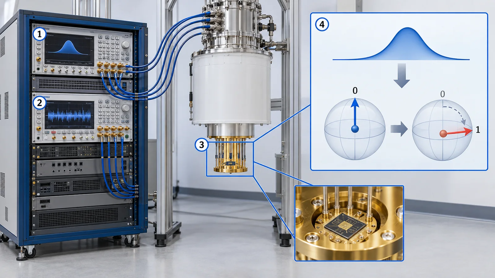
Three-line summary / what to know first / where this sits in the series
What is a gate? The difference from a classical logic gate
Single-qubit gates: rotating the arrow (X, Y, Z, H, S, T)
Combining gates: H, Z, H makes an "invisible change" visible
How to read a quantum circuit diagram
Two-qubit gates: CNOT and how to make entanglement
Measurement: how to measure in another direction
Universal gate sets: a few gates, any computation
What running a circuit means: depth, width, repetition and accumulating errors
A gate is a physical pulse: a materials engineer's view
How to read evaluations and standards
Glossary
References (primary sources)
Claim-to-source audit

Notation used in this article

Sourced = stated in a published source (link given)
Our calculation = a value this article computed or checked from stated assumptions
Not yet confirmed = standards under development, company plans and other items that are not settled
Our own reading for materials engineers is marked as commentary; inference is shown in bold. Every analogy comes with a note on where the analogy breaks down.

How to read the numbers in this article

The matrices, states, probabilities and success rates in Chapters 3 to 9 are our own illustrative calculations, not measurements from a real device. The numbers in the table of Chapter 10 are values each paper reported under its own conditions; they are not meant for ranking devices of different technologies. For standards (ISO/IEC, IEEE) we confirmed only the title, scope and status, not the text. This field moves fast, so devices and standards carry a check date (16 October 2026).

1. Three-line summary / what to know first / where this sits in the series

A quantum gate is an operation that rotates the arrow: X swaps north and south, H tips a north-pointing arrow down to the equator, and Z turns an arrow on the equator by a half-turn. Every gate is reversible Sourced [Ref. 1]
A quantum circuit is a diagram of gates in time order: each horizontal line is one qubit, time runs from left to right, boxes and the ●⊕ symbol are gates, and the meter symbol is a measurement. H and CNOT together can make two qubits "one unit" (entanglement) Sourced [Refs. 1, 14]
A few gates can build any computation: "all single-qubit gates plus CNOT" is exactly universal, and a finite set such as H, T and CNOT can approximate anything to any precision. On real machines gate errors accumulate, so the error rate sets how long a circuit can be Sourced [Refs. 2-4]

What to know before reading

We use the arrow picture from "Quantum Computing Fundamentals" (north pole = 0, south pole = 1, tilted = superposition), together with measurement (measuring gives 0 or 1) and interference (adding waves). If you have not read it, the necessary parts are briefly explained again. Formulas are kept to a minimum, and harder material is tucked into folded "More detail" sections.

Where this sits in the series

This is the article to read after "Quantum Computing Fundamentals". Then come "Coherence and Fidelity" (the yardsticks for gate accuracy) and "Quantum Algorithms" (what to do with the gates). Error correction, technology-specific articles, and software and cloud access are covered in their own articles in the series.

2. What is a gate? The difference from a classical logic gate

Classical computers are built from logic gates (AND, OR, NOT and so on). An AND gate takes two inputs and gives one output: it outputs 1 only when both inputs are 1. The important point is that AND cannot be undone. If the output is 0, you can no longer tell whether the input was "00", "01" or "10". Information has been thrown away.

Quantum gates are different. A quantum gate changes the state of qubits and can always be undone. The number of qubits going in and coming out is also the same. Inside, a quantum gate "rotates the arrow in the sphere about some axis", and rotating the other way restores the original state Sourced [Ref. 1].

Fig. 2 Conceptual diagram (vector drawing). A classical logic gate (AND has two inputs and one output, so information is lost) versus a quantum gate (reversible). The table is the AND truth table; the diagram is for explanation.

A stumbling block: a "quantum gate" is not a quantum version of classical AND or OR

You cannot turn classical AND directly into a quantum gate (it is irreversible). When a quantum computation needs something AND-like, it uses, for example, the Toffoli gate (Chapter 6), which keeps the inputs so that it can be undone. Where the analogy breaks down: the word "gate" is borrowed from classical circuits; inside, a quantum gate is a "rotation of the arrow" (our commentary).

3. Single-qubit gates: rotating the arrow (X, Y, Z, H, S, T)

A gate that acts on one qubit is a single-qubit gate. We use the same convention as in the Fundamentals article: an arrow in a sphere with the north pole as "0" and the south pole as "1". Here is how three representative gates move the arrow.

Fig. 3 Conceptual diagram (vector drawing). How the X, H and Z gates move the arrow (the standard correspondence in the textbook [Ref. 1]). The sphere is drawn as in the Fundamentals article; the x axis points toward the lower left. The axes and results were checked numerically by us.

Gate	Motion of the arrow (axis and angle)	A north-pointing (0) arrow becomes	How to remember
X	180° about the x axis	south (1)	Classical NOT: swaps 0 and 1
Y	180° about the y axis	south (1) (its heading also changes)	Like X, but a different axis
Z	180° about the z axis	still north (only the phase changes)	Turns an arrow on the equator by a half-turn
H (Hadamard)	180° about the axis halfway between x and z	the equator (+x direction)	Creates or undoes a superposition
S	90° about the z axis	still north	"Half" of Z (S twice gives Z)
T	45° about the z axis	still north	"Half" of S (T twice gives S)

Our calculation. We wrote each gate as a matrix, applied it to |0⟩, |1⟩ and |+⟩ (the +x direction on the equator), and confirmed numerically that the arrow ends where the table says, and that S² = Z, T² = S, H·Z·H = X and H·X·H = Z. The gate definitions follow the textbook [Ref. 1] and the Qiskit gate list [Ref. 15] Sourced.

Common misconception: "the Z gate does nothing" is wrong

Apply Z to a north-pointing (0) arrow and it does not move; measuring gives the same result. So it is tempting to say "Z does nothing", but it does act on an arrow on the equator (a half-turn). The phase is merely invisible to direct measurement. As Chapter 4 shows, placing other gates around it turns the difference into "0 or 1".

Axis and angle decide every gate

Any single-qubit gate can be written as three rotations done in turn, about the z, y and z axes (apart from an overall phase) Sourced [Refs. 1, 2]. So a single-qubit gate is determined by "which axis, and how many degrees". In a real machine this rotation is produced by the shape, length and phase of a pulse (Chapter 10).

More detail: gates as matrices (safe to skip)

A single-qubit gate can be written as a 2×2 table (a matrix). For example X is the matrix that swaps the 0 and 1 entries, and H has the factor 1/√2 times the two rows (1, 1) and (1, −1) [Ref. 1]. Multiplying a qubit state (α, β) by the matrix gives the new state. Applying H to |0⟩ = (1, 0) gives (0.7071, 0.7071), that is, 50% each of 0 and 1 (Our calculation). Quantum gates are reversible because these matrices are unitary (their inverses are easy to write down) [Ref. 1].

4. Combining gates: H, Z, H makes an "invisible change" visible

Let us check what "Z changes only the phase" means with an example. Apply H, then Z, then H to a north-pointing (0) arrow. Following the arrow:

Fig. 4 Chart including our calculation (vector drawing). Following the arrow through H, Z, H, which together equal X. We confirmed H·Z·H = X by matrix arithmetic (the relation is also in the textbook [Ref. 1]).

After H: the north-pointing arrow lies on the equator in the +x direction (measuring gives 50% each of 0 and 1)
After Z: it turns to the other side of the equator (−x). Measuring still gives 50% each, so the measurement probabilities have not changed (only the phase has)
After H again: the −x arrow becomes south-pointing (1). Measuring now always gives 1

So H, Z, H together do the same job as X (swapping north and south). Z's "invisible change" was turned by the last H, through interference, into a difference between "0 and 1" Our calculation (H·Z·H = X confirmed numerically by matrices).

A stumbling block: why does a phase difference become a 0/1 difference?

As Chapter 5 of the Fundamentals article showed, applying H twice makes the waves of the two paths reinforce or cancel. If Z sits between them, the sign of the wave on one path flips, so the side that reinforces and the side that cancels are swapped. This is the power of interference, and quantum algorithms use such swaps skilfully to boost the waves of the right answer (see "Quantum Algorithms").

5. How to read a quantum circuit diagram

The standard way to write a quantum computation is a quantum circuit diagram. Read it as follows Sourced [Refs. 1, 14].

Fig. 5 Conceptual diagram (vector drawing). How to read a circuit diagram. This circuit makes an entangled (Bell) state and measures it. The notation follows the common style of IBM Quantum Learning and Qiskit [Refs. 14, 15].

A stumbling block: a horizontal line is "time", not a wire

It is tempting to read the horizontal lines as wires in an electrical circuit, but the lines in a quantum circuit diagram show a qubit progressing through time. A gate is "an operation at one moment" on that line. The vertical line of a CNOT means that the two qubits "are involved at that moment, together". Where the analogy breaks down: real machines do contain wiring, but it is a different thing from the lines of the diagram (Chapter 10).

Qubit numbering: some software shows it reversed

When there are several qubits, the way results are written (such as "01") can be left-right reversed between textbooks and software. For example, when Qiskit shows bits as a string it writes bit 0 at the right end (little-endian) [Ref. 13]. The figures and expressions in this article follow the textbook order (q0 at the left), so when comparing with software output, check the ordering convention Sourced [Ref. 13].

6. Two-qubit gates: CNOT and how to make entanglement

If you only apply gates to each qubit separately, the qubits stay independent forever. What makes qubits interact is a two-qubit gate. The representative one is the CNOT (controlled-NOT) gate, which flips the "target" qubit (applies X to it) only if the "control" qubit is 1 Sourced [Ref. 1].

Fig. 6 Conceptual diagram (vector drawing). The CNOT truth table and the H-then-CNOT route to a Bell state. The state expressions are the standard textbook result [Ref. 1], which we checked by matrix arithmetic.

As the figure shows, putting qubit q0 into a superposition with H and then applying CNOT gives an entangled state (a Bell state) in which only "00" and "11" overlap. Measuring it gives "00" or "11" with equal probability (Our calculation: confirmed by matrices that the result is (|00⟩ + |11⟩)/√2).

Common misconception: "CNOT can copy a quantum state" is wrong

CNOT can copy a state known to be 0 or 1 (north or south) onto another qubit. Applied to a tilted arrow, however, it produces not a copy but an entangled state. In our calculation, CNOT applied to |+⟩|0⟩ gave (|00⟩ + |11⟩)/√2, which is a different state from two |+⟩ side by side (all four components equal to 0.5) (Our calculation). This agrees with the no-cloning theorem [Ref. 1] (Fundamentals article, Chapter 7).

Gate	Qubits	What it does	Worth remembering
CNOT (CX)	2	Flips the target if the control is 1	The basic gate for making entanglement; the keystone of universal sets (Chapter 8)
CZ	2	Flips the phase (makes the sign −1) only when both are 1	CZ = H, CNOT, H (H before and after the target). Many devices run it directly
SWAP	2	Exchanges the states of two qubits	Can be built from three CNOTs. Used between qubits that are not directly connected
Toffoli (CCNOT)	3	Flips the target if both controls are 1	Implements classical AND in a reversible form

Our calculation. We checked, with matrices and over all inputs, that CZ = (I⊗H)·CNOT·(I⊗H), that SWAP equals three CNOTs with alternating direction, and the Toffoli truth table (of the eight inputs, only the two with both controls 1 change). The definitions follow the textbook [Ref. 1] and the Qiskit gate list [Ref. 15] Sourced.

A stumbling block: "control" and "target" do not mean one-way influence

CNOT looks as if "the control commands the target", but when the control qubit is in a superposition, both end up entangled. It is not that only the control affects the target; the two become one state together. "Control" and "target" are just names used when reading the truth table (our commentary).

7. Measurement: how to measure in another direction

At the end of a circuit the qubits are measured. The standard measurement in a circuit diagram asks "north or south?" (0 or 1?), which is a measurement in the computational basis. The result becomes a classical bit.

What if you want to measure along the equator, say in the +x direction? The measurement direction is usually fixed by the hardware, so you first rotate the arrow with a gate so that it points north or south, and then measure. For example, placing H before the measurement turns a +x arrow into north and a −x arrow into south, giving a measurement of the x direction Sourced [Ref. 1].

Fig. 7 Conceptual diagram (vector drawing). Placing H before the measurement turns it into an x-direction measurement (the change of basis in the textbook [Ref. 1]). The results in the figure were checked by matrix arithmetic.

Measurement cannot be undone: measuring fixes the arrow to 0 or 1, and the original state does not return (Fundamentals article, Chapter 4)
Sometimes you measure mid-circuit: not only at the end, but also in the middle, using the result to change later gates (important in quantum error correction; see our article on error correction and the surface code). OpenQASM 3 is designed as a language that can describe such real-time classical control (control flow) Sourced [Ref. 12]
Results are probabilistic: one measurement gives just a 0 or a 1, so the same circuit is run many times (shots) and the ratio is estimated

8. Universal gate sets: a few gates, any computation

Quantum gates come in endless varieties with continuous rotation angles. A real machine cannot offer them all. So, does a small set of gates suffice, with the rest built by combination? The answer is yes, and such a set is called a universal gate set.

Fig. 8 Conceptual diagram (vector drawing). A sorting of universal gate sets, a conceptual diagram based on the results of Barenco et al. [Ref. 2], Boykin et al. [Ref. 3], Dawson and Nielsen [Ref. 4] and Aaronson and Gottesman [Ref. 5].

An exactly universal set: Barenco and colleagues showed that "all single-qubit gates" plus "CNOT" is universal (any operation on any number of qubits can be written as a composition of these) Sourced [Ref. 2]. DiVincenzo showed that two-qubit gates are enough for universality Sourced [Ref. 17]
A finite set that approximates: Boykin and colleagues showed that H, T (the π/8 gate) and CNOT form a universal and fault-tolerant set Sourced [Ref. 3]. According to Dawson and Nielsen's review, the Solovay–Kitaev algorithm approximates any single-qubit gate to precision ε by a sequence of gates from a finite set, and the number of gates it outputs is O(log^3.97(1/ε)) Sourced [Ref. 4]. So raising the precision makes the gate count grow only polynomially in the number of digits
Clifford circuits can be simulated classically: circuits of CNOT, H and the phase gate (S) alone (Clifford circuits) can be simulated efficiently on a classical computer (the Gottesman–Knill theorem) Sourced [Refs. 5, 16]. Adding the T gate makes the set universal

A stumbling block: "universal" does not mean "fast"

Universal means "any quantum computation can be built from this set". It does not mean the construction is short or fast. The number of gates needed differs enormously from problem to problem. It is also known that on error-corrected machines rotation gates such as T are particularly expensive to make (our commentary; see our article on logical qubits and fault-tolerant computing).

9. What running a circuit means: depth, width, repetition and accumulating errors

(1) Words for the size of a circuit

Width: the number of qubits used
Depth: the number of gate layers in time (gates that can run at once count as one layer)
Gate count: the total number of gates, with special attention to the number of two-qubit gates (two-qubit gates usually have larger errors than single-qubit gates; as a reported example, hyperfine qubits in ions reached 99.9934% for single-qubit gates and 99.9% for two-qubit gates [Ref. 19] Sourced)
Shot: one repetition of running and measuring the same circuit

The Bell-state circuit of Chapter 5 has width 2 and depth 2 (H and CNOT).

(2) Errors in each gate accumulate

On a real machine every gate adds a small error. If the error rate per gate is ε and there are N gates, a rule of thumb for the probability that the circuit finishes without a single error is (1 − ε)^N (a simple estimate assuming independent errors).

Fig. 9 Chart including our calculation (vector drawing). A rule-of-thumb success probability (1−ε)ᴺ of a whole circuit versus the number of operations N, for per-gate error rate ε. It is our own illustrative calculation, not a value for any specific device.

Error rate per gate ε	N = 10	N = 100	N = 1,000	N = 10,000
1% (10⁻²)	90.4%	36.6%	about 0.004%	almost 0
0.5% (5×10⁻³)	95.1%	60.6%	0.7%	almost 0
0.1% (10⁻³)	99.0%	90.5%	36.8%	about 0.005%

Our calculation. We computed (1 − ε)^N. It is a simple rule of thumb that treats errors as independent and any single error as failure. Real errors have types (bit flips, phase disturbances, leakage out of the qubit states) and correlations, so reality will not follow it exactly. At N = 1/ε the success probability is about 37% (1/e).

What this calculation teaches: "how many operations you can run" is set almost entirely by the error rate

With an error rate of 0.1%, success falls to 37% after about 1000 gates. Cutting the error rate by a factor of ten lengthens the usable circuit by about a factor of ten. The standard understanding in the field is that the long circuits needed for useful quantum computation require not just a lower error rate but quantum error correction (our commentary; see our article on error correction and the surface code). How to measure gate error rates is covered in "Coherence and Fidelity".

10. A gate is a physical pulse: a materials engineer's view

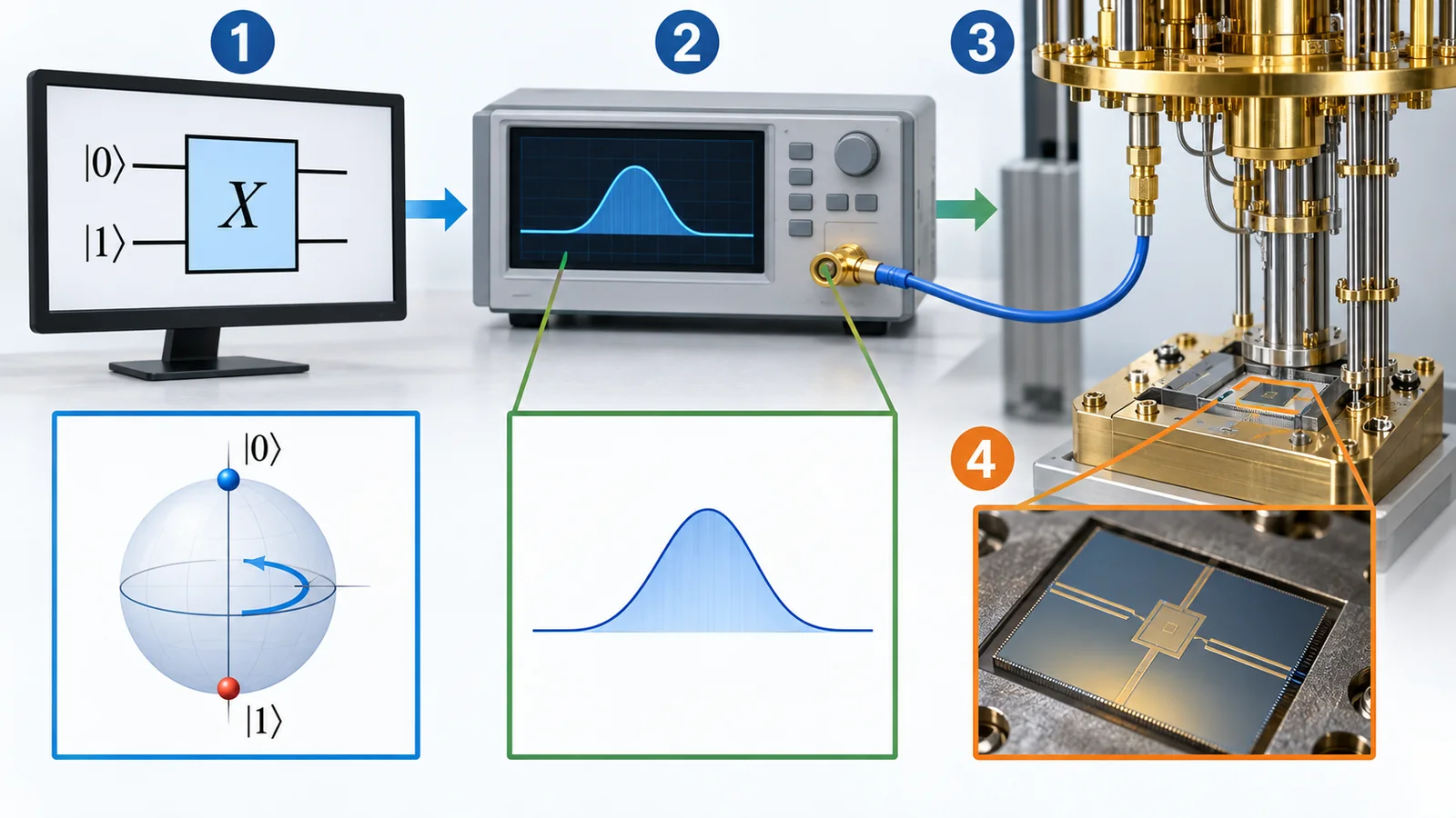
So far a "gate" has been an abstract operation in our heads. On a real machine a gate is sent to the qubit as an electrical or optical "pulse", and the arrow turns as a result. The figure below sets out the steps from the abstract circuit diagram to the actual pulse.

**Fig. 10. Conceptual illustration generated with ImageGen.** The mathematical gate, control pulse and physical device are three distinct layers. The physical operation behind a symbol depends on the hardware platform. Not an actual product, facility, dimensional specification or measurement. Distinguish enlarged models from full-scale scenes.

View original SVG, values and sources

Original SVG reference: Conceptual diagram (vector drawing). A conceptual diagram of the steps by which a gate becomes a physical operation. The examples follow the reviews [Refs. 6-10] and the OpenQASM 3 specification [Ref. 11]; they are not specifications of any device.

On the software side, a circuit is written with abstract gates such as H and CNOT, and a compiler (transpiler) rewrites it into the gates the real machine can perform directly, its native gates. Qiskit's documentation explains that circuits are built from abstract operations without fixing an implementation, and the compiler chooses a good decomposition Sourced [Ref. 15]. The OpenQASM 3 specification also has a section on the relation between its built-in gates and hardware-native gates Sourced [Ref. 11].

(1) What the gate physically is in each technology, with reported gate times and accuracies

The table lists values reported in each paper under its own conditions. Technologies differ in gate time and in how accuracy is measured, so this table is not for ranking.

Technology (report)	What the gate physically is	Reported gate time	Reported accuracy (conditions)
Superconducting Google Quantum AI, 105-qubit processor (2024) [18]	Microwave XY rotations and virtual Z rotations. Two-qubit: CZ gate	XY rotation 25 ns, CZ 42 ns. Mean T₁ 68 µs, T_2,CPMG 89 µs	The paper shows error probabilities as distributions in a figure rather than as numbers in the text (we did not confirm numbers)
Superconducting Sung et al., tunable coupler (2021) [32]	CZ gate and ZZ-free iSWAP gate	Not confirmed here	Two-qubit interaction fidelities: CZ 99.76 ± 0.07%, iSWAP 99.87 ± 0.23%. The paper says these are close to the T₁ limit
Trapped ion Ballance et al. (2016), ⁴³Ca⁺ hyperfine qubits, room-temperature trap [19]	Laser-driven single- and two-qubit gates	Two-qubit gate time varied from 3.8 µs to 520 µs to study the speed/fidelity trade-off	Single-qubit 99.9934(3)%, two-qubit 99.9(1)%
Neutral atom Evered et al. (2023), ⁸⁷Rb atoms in an optical-tweezer array [21]	Two-qubit gate using Rydberg excitation by laser	Not confirmed here	Two-qubit 99.5% (up to 60 atoms in parallel; evaluated by several methods based on repeated gates)
Silicon spin Xue et al. (2022), isotopically enriched ²⁸Si/SiGe double quantum dot [20]	Single-qubit by microwaves, two-qubit CPHASE by an electrical pulse. Z rotations by updating the reference phase (virtual Z)	The idle gate and the CPHASE in the gate set were set to 100 ns	Single- and two-qubit all above 99.5% (gate set tomography)

Sourced (statements in each paper; Refs. 18-21, 32). The arrangement is our commentary. Cells marked "not confirmed" are values we could not confirm from the papers within the scope of this survey.

A stumbling block: the gap between ns and µs is not a ranking of technologies

Looking at a superconducting two-qubit gate (42 ns) and an ion two-qubit gate (several µs to hundreds of µs), it is premature to read "superconducting is a thousand times faster". A gate time means something only against the qubit's coherence time ("Coherence and Fidelity"), and even within one technology speed and accuracy can be traded off. Ballance and colleagues varied the two-qubit gate time from 3.8 to 520 µs to study that relation [Ref. 19]. Always read numbers together with their conditions (our commentary).

**Fig. 11. Conceptual illustration generated with ImageGen.** A scene of control cables attached to a box holding a qubit chip. Gate accuracy depends on cables, packaging and materials too. It does not depict any real facility or product. Not an actual product, facility, dimensional specification or measurement. Distinguish enlarged models from full-scale scenes.

A materials engineer's view 1: the ceiling on gate accuracy is the qubit's lifetime, that is, the materials

A gate has to finish before the qubit's lifetime runs out. The longer a gate takes, the more errors the finite lifetime adds in the meantime. Sung and colleagues state that the fidelities of their CZ and iSWAP gates on superconducting qubits (99.76 ± 0.07% and 99.87 ± 0.23%) are close to the limit set by the qubit's T₁ Sourced [Ref. 32]. At that point however far control is polished, the materials (the qubit's lifetime) set the rest. The quality of the materials a qubit is made of becomes the upper limit of gate accuracy (our commentary; "Coherence and Fidelity" covers the relation between time and error).

A materials engineer's view 2: how precisely you can "make qubits differ" decides gate collisions

In a fixed-frequency superconducting qubit, the frequency is set by the thickness and area of the insulating film of the Josephson junction. As qubits multiply, some pairs end up with frequencies too close, so that gates interfere: frequency crowding becomes a problem. Hertzberg and colleagues adjusted qubit frequencies after fabrication with a laser, improved the precision of setting frequencies by nearly a factor of ten, and showed with statistical modelling that without tuning the probability of finding a collision-free lattice quickly approaches zero Sourced [Ref. 30]. Work to reduce the variation of junction resistance across a wafer has also been reported [Ref. 31].

For a materials engineer, a process that makes an extremely thin oxide film of reproducible thickness and area across the whole wafer determines gate quality once the number of qubits grows (our commentary; for atomic layer deposition and film growth see our articles on atomic layer deposition and on materials and fabrication for quantum computers).

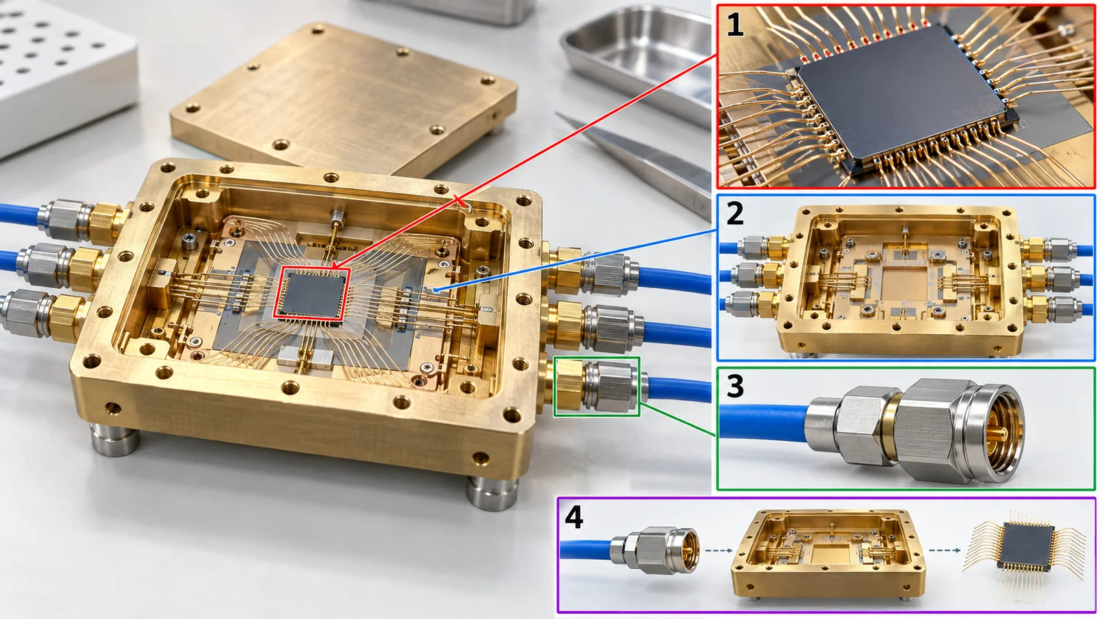
A materials engineer's view 3: wiring, packaging and substrates that carry the gate signal

A gate's pulse travels from room-temperature electronics to the cryogenic qubit through cables, attenuators, connectors, a substrate and a package. If the pulse shape is distorted, noise gets in, or heat flows in, gate accuracy drops. The review of superconducting qubits says that control wiring, read-out amplifiers and on-chip wiring are needed inside the refrigerator, and that the engineering of these is a challenge as the number of qubits grows [Ref. 6]. In silicon spin devices there are examples with gate electrodes on an ²⁸Si-enriched substrate, where electrical pulses run the gates [Ref. 20]. The metals, dielectrics, substrates and bonding materials around a qubit therefore bear directly on gate quality (this contains an inference; our commentary; see our articles on cryogenics and control, and on materials and fabrication for quantum computers).

11. How to read evaluations and standards

The quality of a quantum gate is judged with two "yardsticks": how accurate a single gate is (error rate, fidelity) and how well a whole circuit runs. The first is measured by randomized benchmarking or gate set tomography, the second by quantum volume or application-oriented benchmarks. The table also covers the languages for writing circuits (such as OpenQASM 3) and the standards for terms and performance metrics (checked 16 October 2026).

What is measured	Representative benchmark or evaluation method (name, source)	Standards and guidance (ISO/IEC, IEEE and others)	How to read it
Accuracy of a gate (error rate, fidelity)	Randomized benchmarking (Magesan et al., 2011) [22]. Gate set tomography (Blume-Kohout et al., 2017: showed that operations on a trapped-ion qubit satisfy a fault-tolerance threshold stated in the diamond norm) [29] Sourced	Could not be confirmed (IEEE P7131 has a working group on performance metrics and benchmarking, but we found no published standard) [26] Not yet confirmed	Blume-Kohout et al. state that the "error rate" of randomized benchmarking is not sensitive to all errors and cannot be compared directly with diamond-norm thresholds [29]. Check which operation the value is for and how it was measured
Whole-circuit performance	Quantum volume (Cross et al., 2019) [23]; randomized benchmarking with mirror circuits (Proctor et al., 2022) [27]; application-oriented benchmarks (Lubinski et al., 2023) [28] Sourced	Could not be confirmed (as above)	No single metric expresses superiority for every use; each measures something different
Describing a circuit (language)	OpenQASM 3 (Cross et al., 2022), proposed as a language that can describe real-time classical control (control flow), timing, gate modifiers and more [12] Sourced	The OpenQASM 3 specification (openqasm.com) [11]. We could not confirm it as an ISO/IEC or IEEE standard Sourced	The specification is public but is not an international standard. Gate names and bit-ordering conventions can differ between software [13]
Terms (words for gates and circuits)	— (terminology, not evaluation)	ISO/IEC 4879:2024 "Information technology — Quantum computing — Vocabulary" (edition 1, May 2024, IEC/ISO JTC 3) [24] Sourced / IEEE P7130 "Standard for Quantum Technologies Definitions" (on IEEE's page an active PAR, that is, a project under development; PAR approved 23 September 2021) [25] Not yet confirmed	A vocabulary, not a standard that decides pass or fail for gate performance. We have not read the texts and state none of their definitions
Gate time and speed	Reported individually in each paper (the table in Chapter 10 of this article)	Could not be confirmed (we found no standard reporting format)	Conditions differ between technologies. Read time against the coherence time

The arrangement of this table is our own organisation (Our calculation). The ISO number, title and date were checked on ISO's committee page and the IEEE status on IEEE SA's pages (checked 16 October 2026). The OpenQASM 3 specification and Qiskit documents were checked within what the public pages state. Standard texts are paid or unread, so we limit ourselves to title and scope.

Reading notes (for materials engineers)

"99.9% fidelity" alone does not say what it means: check whether it is a single- or two-qubit gate, for how many qubits, average or best, and how it was measured (randomized benchmarking, tomography and so on)
A randomized-benchmarking number does not reflect every kind of error: Blume-Kohout et al. point out that its "error rate" cannot be compared directly with the fault-tolerance threshold (diamond norm) [Ref. 29]
Do not rank gate times or accuracies of devices of different technologies: the conditions differ, and the trade-off between speed and accuracy differs by technology (table in Chapter 10)
Check whether a standard is a recommendation or a requirement: ISO/IEC 4879 is a vocabulary, OpenQASM 3 is a public specification, and IEEE P7130 and P7131 are projects under development. For any claim of "compliance", ask which standard and which clause

12. Glossary

Quantum gate: An operation that rotates a qubit's arrow. It is reversible.

Quantum circuit: A diagram of quantum gates and measurements in time order (or the procedure it describes).

Logic gate: A classical AND, OR, NOT and so on. Many cannot be undone.

X gate: Swaps 0 and 1: north and south (180° about the x axis).

Z gate: Flips the phase: 180° about the z axis. Leaves north- and south-pointing arrows where they are.

H (Hadamard) gate: Tips a north-pointing arrow down to the equator. Creates or undoes a superposition.

S gate, T gate: Rotations of 90° and 45° about the z axis. S twice gives Z; T twice gives S.

CNOT (controlled-NOT): A two-qubit gate that flips the target if the control is 1. It makes entanglement.

CZ: A two-qubit gate that flips the phase only when both are 1.

SWAP: A gate that exchanges the states of two qubits.

Toffoli (CCNOT): A three-qubit gate that flips the target if both controls are 1.

Unitary: A reversible transformation (it keeps total probability). Quantum gates are unitary.

Bell state: The typical entangled state in which two qubits are a superposition of "00" and "11".

Universal gate set: A set of gates from which any quantum computation can be built (including by approximation).

Clifford gates: H, S, CNOT and so on. Circuits made only of them can be simulated efficiently on a classical computer.

Solovay–Kitaev: A method to approximate any gate accurately with a sequence of gates from a finite set.

Native gate: A gate the device can perform directly in one operation.

Transpiling (compiling): Rewriting an abstract circuit into a sequence of the device's native gates.

Depth, width: The number of time layers of a circuit; the number of qubits used.

Shot: One repetition of running and measuring the same circuit.

Fidelity: A number showing how close an actual operation is to the ideal one (closer to 1 is better).

Randomized benchmarking: A method that finds the error rate per operation using random sequences of operations.

Gate set tomography: A measurement method that characterises the behaviour of a whole set of gates in detail.

OpenQASM: A publicly specified language for writing quantum circuits.

13. References (primary sources)

Nielsen M. A., Chuang I. L. Quantum Computation and Quantum Information, Cambridge University Press (10th anniversary edition, 2010) (book page) — cambridge.org
Barenco A. et al. "Elementary gates for quantum computation", Phys. Rev. A 52, 3457–3467 (1995), DOI 10.1103/PhysRevA.52.3457 — doi.org/10.1103/PhysRevA.52.3457
Boykin P. O. et al. "On Universal and Fault-Tolerant Quantum Computing", arXiv:quant-ph/9906054 (1999) — arxiv.org/abs/quant-ph/9906054
Dawson C. M., Nielsen M. A. "The Solovay-Kitaev algorithm", Quantum Inf. Comput. 6, 81–95 (2006), arXiv:quant-ph/0505030 — arxiv.org/abs/quant-ph/0505030
Aaronson S., Gottesman D. "Improved simulation of stabilizer circuits", Phys. Rev. A 70, 052328 (2004), DOI 10.1103/PhysRevA.70.052328 — doi.org/10.1103/PhysRevA.70.052328
Krantz P. et al. "A quantum engineer's guide to superconducting qubits", Appl. Phys. Rev. 6, 021318 (2019), DOI 10.1063/1.5089550 — doi.org/10.1063/1.5089550
Bruzewicz C. D. et al. "Trapped-ion quantum computing: Progress and challenges", Appl. Phys. Rev. 6, 021314 (2019), DOI 10.1063/1.5088164 — doi.org/10.1063/1.5088164
Henriet L. et al. "Quantum computing with neutral atoms", Quantum 4, 327 (2020), DOI 10.22331/q-2020-09-21-327 — doi.org/10.22331/q-2020-09-21-327
Slussarenko S., Pryde G. J. "Photonic quantum information processing: A concise review", Appl. Phys. Rev. 6, 041303 (2019), DOI 10.1063/1.5115814 — doi.org/10.1063/1.5115814
Burkard G. et al. "Semiconductor spin qubits", Rev. Mod. Phys. 95, 025003 (2023), DOI 10.1103/RevModPhys.95.025003 — doi.org/10.1103/RevModPhys.95.025003
OpenQASM "OpenQASM 3.0 Specification" (specification pages; checked 16 October 2026) — openqasm.com/versions/3.0/index.html
Cross A. et al. "OpenQASM 3: A Broader and Deeper Quantum Assembly Language", ACM Trans. Quantum Comput. 3, 12 (2022), DOI 10.1145/3505636 — doi.org/10.1145/3505636
IBM Quantum "Bit-ordering in the Qiskit SDK" (documentation) (checked 16 October 2026) — quantum.cloud.ibm.com/docs/en/guides/bit-ordering
IBM Quantum Learning "Basics of quantum information" (course) (introductory course; consulted for the arrow and circuit-diagram conventions) — quantum.cloud.ibm.com/learning/en/courses/basics-of-quantum-information
IBM Quantum "Circuit library" (Qiskit SDK documentation) (checked 16 October 2026) — quantum.cloud.ibm.com/docs/en/api/qiskit/circuit_library
Gottesman D. "The Heisenberg Representation of Quantum Computers", arXiv:quant-ph/9807006 (1998) — arxiv.org/abs/quant-ph/9807006
DiVincenzo D. P. "Two-bit gates are universal for quantum computation", Phys. Rev. A 51, 1015–1022 (1995), DOI 10.1103/PhysRevA.51.1015 — doi.org/10.1103/PhysRevA.51.1015
Google Quantum AI "Quantum error correction below the surface code threshold", Nature 638, 920–926 (2025), DOI 10.1038/s41586-024-08449-y (arXiv:2408.13687) — doi.org/10.1038/s41586-024-08449-y
Ballance C. J. et al. "High-Fidelity Quantum Logic Gates Using Trapped-Ion Hyperfine Qubits", Phys. Rev. Lett. 117, 060504 (2016), DOI 10.1103/PhysRevLett.117.060504 — doi.org/10.1103/PhysRevLett.117.060504
Xue X. et al. "Quantum logic with spin qubits crossing the surface code threshold", Nature 601, 343–347 (2022), DOI 10.1038/s41586-021-04273-w — doi.org/10.1038/s41586-021-04273-w
Evered S. J. et al. "High-fidelity parallel entangling gates on a neutral-atom quantum computer", Nature 622, 268–272 (2023), DOI 10.1038/s41586-023-06481-y — doi.org/10.1038/s41586-023-06481-y
Magesan E., Gambetta J. M., Emerson J. "Scalable and Robust Randomized Benchmarking of Quantum Processes", Phys. Rev. Lett. 106, 180504 (2011), DOI 10.1103/PhysRevLett.106.180504 — doi.org/10.1103/PhysRevLett.106.180504
Cross A. W. et al. "Validating quantum computers using randomized model circuits", Phys. Rev. A 100, 032328 (2019), DOI 10.1103/PhysRevA.100.032328 — doi.org/10.1103/PhysRevA.100.032328
ISO/IEC "ISO/IEC 4879:2024 Information technology — Quantum computing — Vocabulary" (edition 1, May 2024, IEC/ISO JTC 3; checked on ISO's committee page) — iso.org/standard/80432.html
IEEE SA "IEEE P7130 Draft Standard for Quantum Technologies Definitions" (project page) (active PAR, approved 23 September 2021; checked 16 October 2026) — standards.ieee.org/ieee/7130/10680/
IEEE SA "Quantum Benchmarking Working Group P7131" (page of the working group on quantum computing performance metrics; checked 16 October 2026) — sagroups.ieee.org/7131
Proctor T. et al. "Scalable Randomized Benchmarking of Quantum Computers Using Mirror Circuits", Phys. Rev. Lett. 129, 150502 (2022), DOI 10.1103/PhysRevLett.129.150502 — doi.org/10.1103/PhysRevLett.129.150502
Lubinski T. et al. "Application-Oriented Performance Benchmarks for Quantum Computing", IEEE Trans. Quantum Eng. 4, 1–32 (2023), DOI 10.1109/TQE.2023.3253761 — doi.org/10.1109/TQE.2023.3253761
Blume-Kohout R. et al. "Demonstration of qubit operations below a rigorous fault tolerance threshold with gate set tomography", Nat. Commun. 8, 14485 (2017), DOI 10.1038/ncomms14485 — doi.org/10.1038/ncomms14485
Hertzberg J. B. et al. "Laser-annealing Josephson junctions for yielding scaled-up superconducting quantum processors", npj Quantum Inf. 7, 129 (2021), DOI 10.1038/s41534-021-00464-5 — doi.org/10.1038/s41534-021-00464-5
Kreikebaum J. M. et al. "Improving wafer-scale Josephson junction resistance variation in superconducting quantum coherent circuits", Supercond. Sci. Technol. 33, 06LT02 (2020), DOI 10.1088/1361-6668/ab8617 (title only; text not read) — doi.org/10.1088/1361-6668/ab8617
Sung Y. et al. "Realization of High-Fidelity CZ and ZZ-Free iSWAP Gates with a Tunable Coupler", Phys. Rev. X 11, 021058 (2021), DOI 10.1103/PhysRevX.11.021058 — doi.org/10.1103/PhysRevX.11.021058

14. Claim-to-source audit

Claim in the text	Basis	Category
That quantum gates are rotations of the arrow and are reversible; the definitions of X, Y, Z, H, S, T, CNOT, CZ, SWAP and Toffoli; how to read circuit diagrams; placing H before a measurement to change its direction	Textbook (Nielsen and Chuang), IBM Quantum Learning, the Qiskit gate list Reference 1 https://www.cambridge.org/highereducation/books/quantum-computation-and-quantum-information/01E10196D0A682A6AEFFEA52D53BE9AE Reference 14 https://quantum.cloud.ibm.com/learning/en/courses/basics-of-quantum-information Reference 15 https://quantum.cloud.ibm.com/docs/en/api/qiskit/circuit_library	Sourced
That all single-qubit gates plus CNOT form an exactly universal set; that two-qubit gates are universal	Abstract of Barenco et al. (1995) and title of DiVincenzo (1995) Reference 2 https://doi.org/10.1103/PhysRevA.52.3457 Reference 17 https://doi.org/10.1103/PhysRevA.51.1015	Sourced
That H, T and CNOT form a universal fault-tolerant set; that the Solovay–Kitaev algorithm outputs O(log^3.97(1/ε)) gates	Abstracts of Boykin et al. and of Dawson and Nielsen Reference 3 https://arxiv.org/abs/quant-ph/9906054 Reference 4 https://arxiv.org/abs/quant-ph/0505030	Sourced
That Clifford circuits (CNOT, H, phase gates) can be simulated efficiently on a classical computer (Gottesman–Knill theorem)	Abstracts of Aaronson and Gottesman (2004) and Gottesman (1998) Reference 5 https://doi.org/10.1103/PhysRevA.70.052328 Reference 16 https://arxiv.org/abs/quant-ph/9807006	Sourced
That Qiskit writes bit 0 at the right end of a displayed bit string (little-endian)	Qiskit documentation "Bit-ordering in the Qiskit SDK" Reference 13 https://quantum.cloud.ibm.com/docs/en/guides/bit-ordering	Sourced
That a compiler rewrites a circuit of abstract gates into native gates; the OpenQASM 3 specification and proposal	Qiskit documentation, the OpenQASM 3 specification, abstract of Cross et al. (2022) Reference 15 https://quantum.cloud.ibm.com/docs/en/api/qiskit/circuit_library Reference 11 https://openqasm.com/versions/3.0/index.html Reference 12 https://doi.org/10.1145/3505636	Sourced
Figures in the Chapter 10 table: superconducting (XY rotation 25 ns, CZ 42 ns, T1 68 µs, T2,CPMG 89 µs), CZ 99.76 ± 0.07%, ion (3.8 to 520 µs, 99.9934%, 99.9%), neutral atom 99.5%, silicon spin (100 ns, above 99.5%)	Text, abstracts and supplements of the papers (Google Quantum AI, Sung et al., Ballance et al., Evered et al., Xue et al.) Reference 18 https://doi.org/10.1038/s41586-024-08449-y Reference 32 https://doi.org/10.1103/PhysRevX.11.021058 Reference 19 https://doi.org/10.1103/PhysRevLett.117.060504 Reference 21 https://doi.org/10.1038/s41586-023-06481-y Reference 20 https://doi.org/10.1038/s41586-021-04273-w	Sourced
Overviews of the qubits and gates of each technology (superconducting, ion, neutral atom, photonic, silicon spin)	Review articles on each technology Reference 6 https://doi.org/10.1063/1.5089550 Reference 7 https://doi.org/10.1063/1.5088164 Reference 8 https://doi.org/10.22331/q-2020-09-21-327 Reference 9 https://doi.org/10.1063/1.5115814 Reference 10 https://doi.org/10.1103/RevModPhys.95.025003	Sourced
That post-fabrication laser tuning improved the precision of setting qubit frequencies nearly ten-fold to counter frequency crowding; the title of work improving junction-resistance variation	Abstract of Hertzberg et al. (2021); title only of Kreikebaum et al. (2020) Reference 30 https://doi.org/10.1038/s41534-021-00464-5 Reference 31 https://doi.org/10.1088/1361-6668/ab8617	Sourced
The proposals of randomized benchmarking, gate set tomography, quantum volume, mirror circuits and application-oriented benchmarks; that the RB "error rate" cannot be compared directly with diamond-norm thresholds	Magesan et al., Blume-Kohout et al., Cross et al., Proctor et al., Lubinski et al. Reference 22 https://doi.org/10.1103/PhysRevLett.106.180504 Reference 29 https://doi.org/10.1038/ncomms14485 Reference 23 https://doi.org/10.1103/PhysRevA.100.032328 Reference 27 https://doi.org/10.1103/PhysRevLett.129.150502 Reference 28 https://doi.org/10.1109/TQE.2023.3253761	Sourced
The number, title and date of ISO/IEC 4879:2024 "Information technology — Quantum computing — Vocabulary" (edition 1, May 2024, IEC/ISO JTC 3)	ISO's committee page Reference 24 https://www.iso.org/standard/80432.html	Sourced
That IEEE P7130 is under development (active PAR, approved 23 September 2021); that the IEEE P7131 working group is active and we found no published standard	IEEE SA pages Reference 25 https://standards.ieee.org/ieee/7130/10680/ Reference 26 https://sagroups.ieee.org/7131	Not yet confirmed
The matrix checks (S²=Z, T²=S, H·Z·H=X, H·X·H=Z, CZ=(I⊗H)·CNOT·(I⊗H), SWAP as three CNOTs, the Toffoli truth table, the Bell state, CNOT on \|+⟩\|0⟩) and the success-probability table (1−ε)^N	Our own calculation (Python, NumPy). A simple rule of thumb treating errors as independent and any error as failure. Not the results of any real device	Our calculation
The text of ISO/IEC 4879, the publication state of IEEE P7131, the neutral-atom two-qubit gate duration, the Sung et al. CZ duration, and any comparison of gate performance across technologies	Could not be confirmed from the primary sources available in this survey, so not stated	commentary
Readings such as "Z does nothing is wrong", "the ns versus µs gap is not a ranking", "universal does not mean fast", "materials set the ceiling on gate accuracy", and the analogies with their limits	Our own organisation and commentary based on the published material; not views expressed by the organisations cited	commentary
That Figs. 1 to 11 are explanatory drawings and not observations of real data, and that Figs. 1 and 11 are ImageGen-generated conceptual illustrations	Note in this article	commentary

Last updated: 16 October 2026. Sources are limited to primary material (a textbook, peer-reviewed papers, arXiv papers, official OpenQASM 3 and Qiskit documents, and official ISO and IEEE pages). Values from companies and laboratories are shown as values under each paper's conditions, and we do not rank devices of different technologies. The numerical examples (matrix checks, the success-probability table) are our own illustrative calculations, not results from real devices. We could not confirm the text of the standards, the publication state of IEEE P7131, or some gate times and accuracies from the papers, so we do not state them. All figures are explanatory conceptual diagrams or drawings that include our own calculations; Figs. 1 and 11 are ImageGen-generated conceptual illustrations.

Illustration update: 17 October 2026. References to vector drawings in the article and source tables describe the retained original SVGs. See each current caption for the foreground image format and reading guide. ImageGen illustrations are not measurements or photographs of actual products; original SVGs, values and sources remain available in expandable references.