TECHNOLOGY EXPLAINER
Materials and Fabrication for Quantum Computers
— What sets a qubit's performance is less the circuit diagram than surfaces, interfaces, defects, isotopes and heat
A qubit does not work just because it is built to the drawing. A large part of its performance is decided by questions of materials and manufacturing: a few nanometres of oxide, the surface of a metal film, defects inside the substrate, isotope purity, and the cooling power of the refrigerator. As the materials-engineer keystone of this series, this article follows superconducting qubits in particular and goes through how Josephson junctions are made, loss from two-level systems (TLS), tantalum versus niobium, substrates, quasiparticles and radiation, manufacturing on 300 mm semiconductor foundry lines and the spread it brings, and cryogenic wiring and heat, with diagrams and simple calculations. It asks what limits performance, using published papers and technical reports, and keeps the best laboratory values apart from values that can be reproduced across a chip (checked on 16 October 2026).
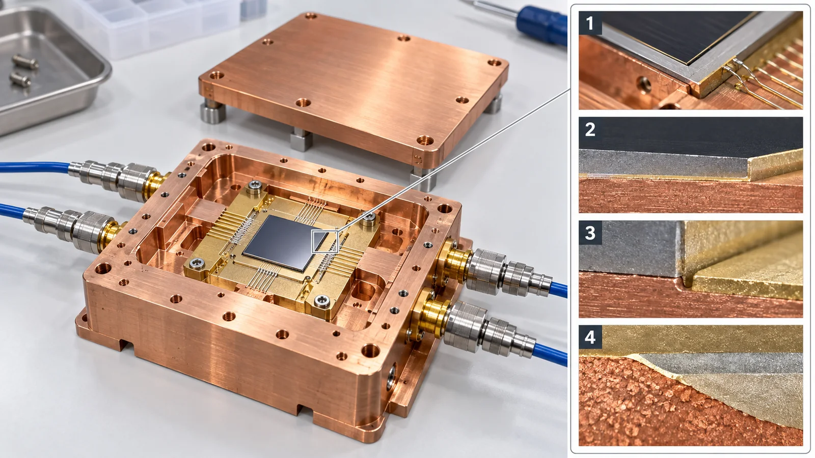
- What it covers: a qubit's lifetime (T1) and the accuracy of its operations are decided to a large extent by surfaces, interfaces, defects, isotopes and heat. In superconducting qubits, a surface oxide only a few nanometres thick plays a large role
- Conclusion: the best T1 for a single qubit reached 1.68 ms (tantalum on high-resistivity silicon, 2025), but the average over a 105-qubit chip is 68 µs, and a 300 mm production line gives just over 100 µs. Between the best value and the value that can be reproduced across a chip there is a gap of more than a factor of ten. Closing it is the job of materials and manufacturing
- The most important point: there is no single culprit for “what limits performance.” In tantalum devices, the loss in the surface dielectric and in the bulk dielectric has been reported to be comparable. The dominant factor differs from device to device, so the core of this field is to measure, separate and then treat each loss
It helps to know that a qubit can be drawn as an arrow from the centre of a sphere to its surface, and that the arrow gets blurred by its surroundings (decoherence). Think of T1 as roughly the time before the arrow falls back to its original direction (a lifetime); see our explainer on coherence and fidelity. Materials terms (oxide film, epitaxial growth and so on) are explained where they appear.
Where this fits in the seriesRead this after our explainers on superconducting qubits, cryogenics and control, and coherence and fidelity, and the whole picture connects. Silicon-28 and its interfaces are covered in our explainer on silicon spin qubits, diamond isotopes in our explainer on quantum sensing, interfaces between nanowires and superconductors in our explainer on topological quantum computing, how thin films are made in our explainer on atomic layer deposition, and inspection techniques in our explainer on nanometrology. This article is the one that cuts across them from a materials engineer's point of view. Electric-field noise at ion-trap surfaces is covered in our explainer on ion traps.
- Why materials decide performance — the length of the ring-down, and losses that add up
- Materials and fabrication of superconducting qubits — junctions, oxides, substrates, spread
- Materials of other approaches — silicon, diamond, ions, topological
- Cryogenic wiring and heat — the budget set by cooling power
- What limits performance — sorting out the factors
- What we could not confirm, and a summary
- How to read evaluations and standards
- Glossary
- References (primary sources)
- Claim-to-source audit
Sourced = stated in a published source (with a link)
Our calculation = a value this article computed from stated assumptions
Not yet confirmed = plans, targets, items under review and so on
Our reading of what this means for materials is marked as commentary. Inference is shown in bold. Company announcements and technical blogs are treated as “company claims.”
Values such as T1 differ from paper to paper in qubit frequency, design, measurement method and whether the figure is an average or a best value. Placing them side by side does not rank them or the approaches. The best value in a laboratory and the performance of a production part are different things. Company announcements are treated as company claims. Some worked examples (participation ratio, frequency, number of cables) use assumed values, and each is stated where it appears.
1. Why materials decide performance — the length of the ring-down, and losses that add up
Start with an everyday feeling
When you strike a bell, the sound rings for a long time. That “length of the ring-down” corresponds to a qubit's T1 (its lifetime). Even if the bell itself is good metal, a loose fitting, rust or a dirty surface makes the ring die away quickly. It is not only the metal's quality inside (the bulk) but also the places it touches (surfaces and interfaces) that decide the ring-down.
A qubit is the same. Place and co-workers write that the relaxation times of superconducting qubits (transmons) are orders of magnitude shorter than the limits set by the bulk properties of the constituent materials, and that the cause appears to lie in uncontrolled surfaces, interfaces and contaminants Sourced [Reference 1]. Siddiqi's review likewise says that going from bulk materials to working devices introduces amorphous films and non-equilibrium excitations (electronic and phononic), and that the resulting dissipation and fluctuations limit state-of-the-art qubits and processors [Reference 6].
Think of losses as a sum
The energy a qubit loses is the sum of the losses at many places in the device. Wang and co-workers showed that the relaxation rate of a transmon is roughly proportional to the fraction of electric-field energy stored in the surface dielectric layers (the surface participation), and said that dielectric loss at material interfaces is a main factor limiting T1 Sourced [Reference 14]. As formulas (our commentary; these are general relations):
- 1/Q = Σ (participation pi × loss tangent tanδi): for each place i, multiply “how much of the electric field reaches it (p)” by “how lossy that material is (tanδ)” and add them up
- T1 = Q ÷ ω = Q ÷ (2π f): the larger Q is, the longer it lasts. f is the qubit frequency
Let us get a feel for the numbers. Take f = 5 GHz (an assumed example). Q = 106 gives T1 of about 32 µs, Q = 107 gives about 320 µs, and Q = 2.5 × 10⁷ gives about 0.8 ms Our calculation. One more. Verjauw and co-workers report the loss tangent of niobium pentoxide, Nb2O5, which forms on niobium surfaces, as tanδ = 9.9 × 10⁻³ [Reference 12]. Suppose 10−4 of the electric-field energy sits in this oxide (an assumed value). Then 1/Q = 10−4 × 9.9 × 10−3 = about 10−6, so Q is about 106, and at 5 GHz T1 is about 32 µs Our calculation. Even an extremely thin film can cut a qubit's lifetime by nearly a factor of ten if its loss tangent is large.
Inside an amorphous oxide film (one without the regular arrangement of a crystal), there are many tiny defects where an atom can “hop” slightly to another position. Because they can switch between two states, they are called two-level systems (TLS). When the energy difference of a TLS happens to match the qubit's energy, the qubit has its energy absorbed. Müller and co-workers' review writes that superconducting circuits made of aluminium or niobium are fundamentally limited by loss from two-level defects in the amorphous oxide that covers them, and that the central question of what those defects really are is still unanswered Sourced [Reference 10]. In other words, the nature of TLS is not yet fully understood, and in practice empirical countermeasures such as reducing, thinning or replacing the oxide are being tried (our summary).
Where does the loss happen? — a cross-section of the device
A transmon is built by making capacitor electrodes from thin metal films on a substrate, with a small Josephson junction between them. The electric field passes through the substrate and the metal surfaces between the electrodes. Loss can occur anywhere the field passes.
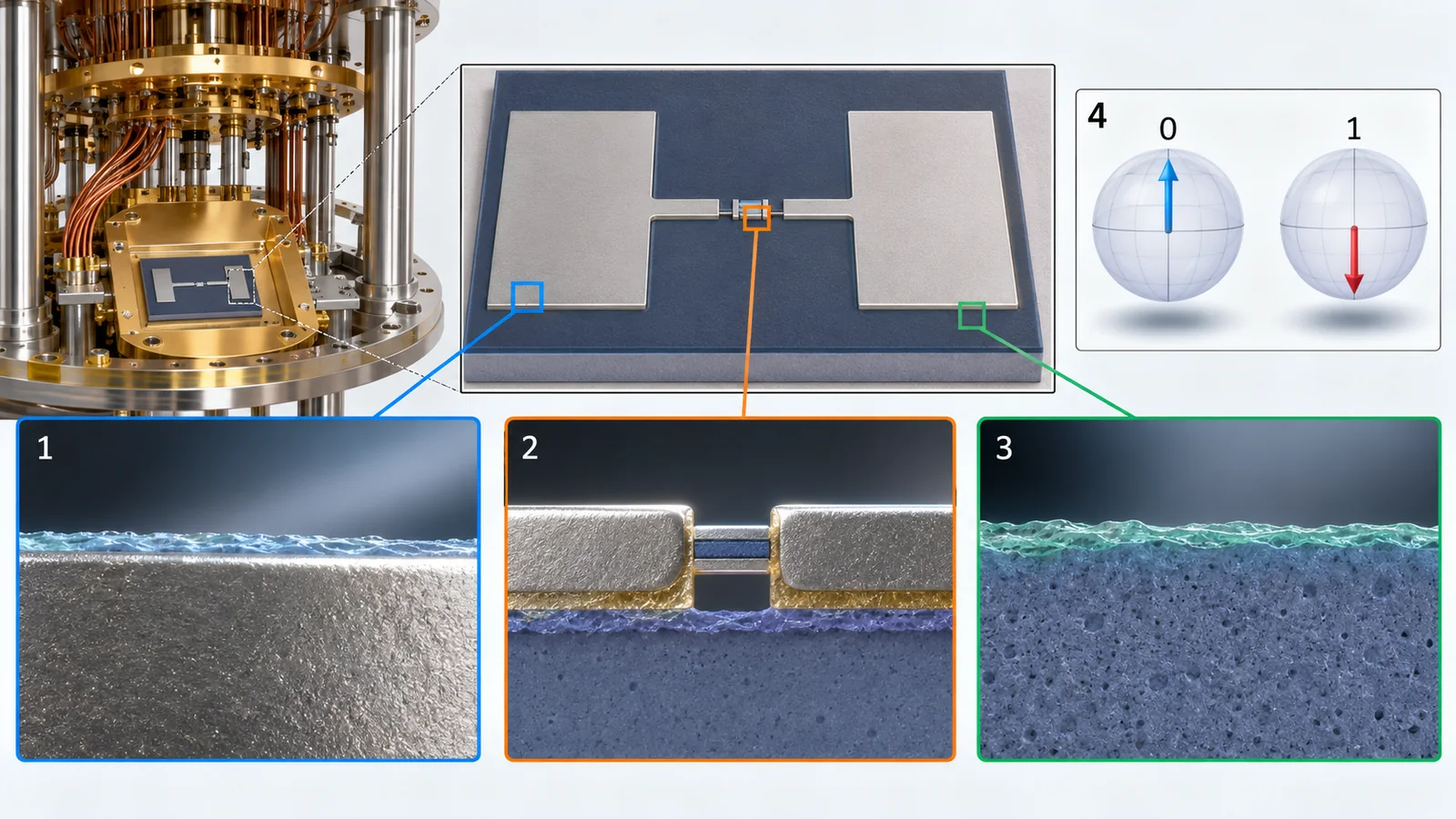
View original SVG, values and sources
Original SVG reference: Concept diagram (vector drawing). Cross-section of a transmon and the places where loss occurs. 1: metal surface (natural oxide); 2: substrate surface (between the electrodes); 3: bulk substrate; 4: interface between metal and substrate, and inside the metal (including quasiparticles); 5: the junction and the oxide and wiring contacts around it. Places the electric field (red dashed lines) passes through are candidates for loss [References 9, 11, 14]. Dimensions and layer thicknesses are illustrative.
| No. | Place | What has been reported (source) | Cautions in reading |
|---|---|---|---|
| 1 | Oxide on the metal surface | The surface oxide of Nb, Nb2O5, has tanδ = 9.9 × 10⁻³ [Reference 12]. Altoé and co-workers report that most non-TLS loss is distributed in the niobium surface oxide [Reference 11] Sourced | Native oxides of Ta, TiN and Al are reported to matter less than the Nb oxide (Bal et al.) [Reference 4] |
| 2 | Substrate surface (silicon oxide and so on) | Altoé and co-workers showed, in niobium-on-silicon resonators, that most TLS loss comes from the silicon surface oxide [Reference 11] Sourced | Other substrates (such as sapphire) may behave differently |
| 3 | Bulk substrate | In Ta-on-sapphire devices the loss is dominated by TLS, with comparable contributions from surface and bulk dielectrics (as stated in the introduction of Bland et al.) [Reference 3]. Bland and co-workers report that moving to high-resistivity silicon markedly lowers bulk substrate loss [Reference 3] Sourced | Without treating both surface and bulk, large gains are unlikely |
| 4 | Metal–substrate interface; inside the metal (quasiparticles) | Crowley and co-workers report, for Ta resonators, that loss is dominated by several kinds of saturable TLS, that both surface and bulk contribute, and that surface TLS can be altered by chemical processing [Reference 13]. Quasiparticles are treated in a later section Sourced | Internal Q of the resonators was 5 to 15 × 106 (comparable to the best qubits) |
| 5 | The Josephson junction and its surroundings | Osman and co-workers describe a patch between junction electrodes and wiring that removes parasitic junctions and so reduces dielectric loss, and a way to make it in a single vacuum cycle [Reference 15]. Bland and co-workers report that low-contamination junction deposition let T2 (Hahn echo) exceed T1 [Reference 3] Sourced | The surroundings of the junction have entered the stage where they decide the lifetime |
The table is our summary (Our calculation). Numbers match Fig. 3. Each value is as stated in the individual paper; devices, substrates, temperatures and photon numbers differ.
Wrong: “if the design drawing is the same, performance is the same wherever it is made.” In fact: the design sets how much of the electric field passes through which place (the participation), but the quality of the material at that place (its loss tangent) is set by deposition, processing and cleaning. For Google's 105-qubit chip, the authors attribute the mean T1 of 68 µs to improved fabrication techniques, participation-ratio engineering and optimisation of circuit parameters Sourced [Reference 22]. Both design and materials are needed.
Materials are normally chosen from property tables (permittivity, loss tangent, thermal conductivity). In a qubit, however, a few nanometres of native oxide, tens of minutes of exposure to air after cleaning, leftover resist and processing damage at the substrate surface matter by orders of magnitude more than the bulk values in the table. Verjauw and co-workers report that, after removing the native oxide of niobium resonators with hydrofluoric acid, exposure to air for 16 minutes gave a loss an order of magnitude lower, with internal Q reaching 7 × 10⁶ at the single-photon level [Reference 12]. “When, in what atmosphere, for how many minutes” is process information that becomes the performance of the material itself (our commentary).
2. Materials and fabrication of superconducting qubits — junctions, oxides, substrates, spread
Superconducting qubits are one of the main approaches in today's quantum computers, and their materials and manufacturing problems are the best studied. Here we look at (1) how the Josephson junction at the heart of the qubit is made, (2) the surface oxide, (3) tantalum, niobium and the substrate, and (4) the spread between junctions, in that order. For how a superconducting qubit works, see our explainer on superconducting qubits. For an overview of the field see the review by Kjaergaard and co-workers [Reference 28], and for a classic review of the materials of superconducting qubits see Oliver and Welander [Reference 8].
2.1 What a Josephson junction is — two superconductors with an extremely thin wall between them
A Josephson junction is a structure with a very thin insulating film sandwiched between two superconductors. Pairs of superconducting electrons (Cooper pairs) pass through this thin wall by “tunnelling.” Kreikebaum and co-workers describe the transmon as “a Josephson junction functioning as a non-linear inductor shunted with a capacitor to form an anharmonic oscillator” Sourced [Reference 18]. The aluminium-based junctions used for qubits have three layers: aluminium (Al), its oxide (AlOx), and aluminium again [References 15, 18].
What does “anharmonic” mean? An ordinary oscillator such as a swing (a harmonic oscillator) has energy steps spaced equally. With equal spacing, an operation that lifts 0 to 1 also acts in the same way on 1 to 2, so you cannot pick out just 0 and 1. The junction makes the spacing slightly uneven. As an analogy, it is like adding “bumps” to the rungs of an evenly spaced ladder so that only the 0 and 1 rungs can be told apart (our own analogy for explanation). Hertzberg and co-workers write that transmons are weakly anharmonic, with transition energies that decrease at higher levels [Reference 17].
Wrong: “qubit performance is poor because of oxide, so remove the oxide.” In fact: the Josephson junction itself uses an oxide film made on purpose (AlOx) as its wall. Without it the qubit does not work. What lowers performance is unintended amorphous oxide where the electric field passes (the native oxide on metal surfaces and the oxide on the substrate surface). What matters is to tell apart “which oxide, and where” (our summary).
2.2 How a junction is made — evaporating from an angle to make an overlap
Aluminium-based junctions have long been made by angled (shadow) evaporation. The origin is the method using a resist “bridge” reported by Dolan in 1977 [Reference 24], and bridge-free methods (such as the Manhattan style) are also used [References 18, 25]. The flow is shown in Fig. 4.
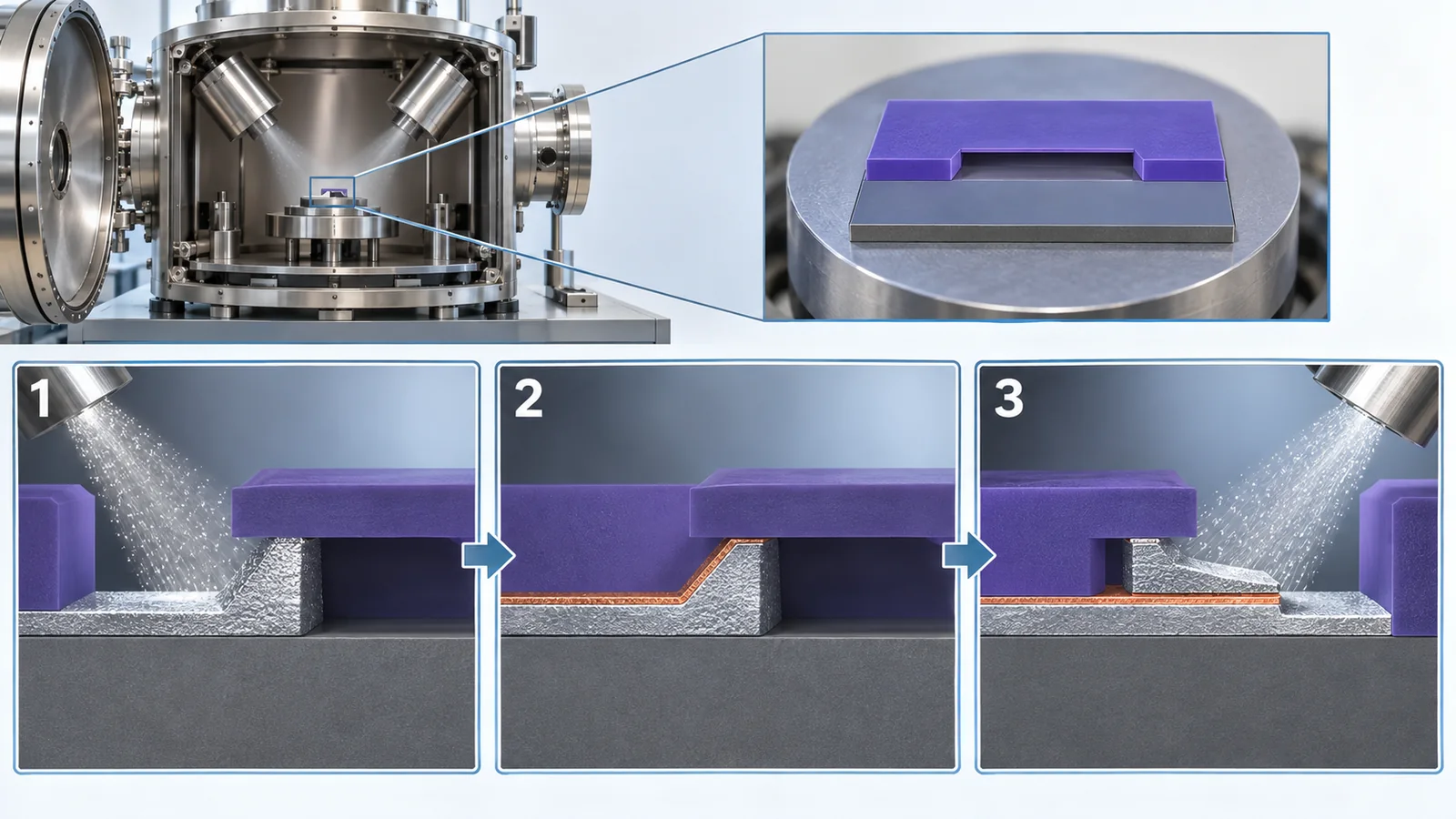
View original SVG, values and sources
Original SVG reference: Concept diagram (vector drawing). The flow of angled (double-angle) evaporation. 1: open a window in two layers of resist. 2: evaporate aluminium from an angle for the first time. 3: without breaking vacuum, admit oxygen to form a thin oxide (AlOx) on the surface. 4: evaporate again from the opposite angle. The small area where the two films overlap becomes the Josephson junction. Afterwards the resist and the excess metal on it are dissolved away (lift-off) [References 18, 24, 25]. Dimensions and angles are illustrative.
What matters to a materials engineer is step 3, the oxidation, and the dimensions. The tunnelling current depends extremely sensitively (exponentially, a general physical fact) on the thickness of the wall, so slight differences in oxidation pressure, time and temperature become differences in the junction resistance (Rn) (our commentary). Kreikebaum and co-workers report that when 64 chips of 1 × 1 cm were made from a 150 mm wafer by simply transplanting a recipe optimised for single devices, the room-temperature tunnelling resistance drifted by ±30% across the wafer; in a systematic study of 38 wafers they optimised uniform ashing, ultrasonically assisted resist development and dynamic oxidation (oxidation with gas flowing continuously) Sourced [Reference 18].
Another trick is removing parasitic junctions. Osman and co-workers state that, for shadow-evaporated aluminium junctions, a “patch” joining the junction electrodes to the surrounding wiring is normally made in a separate lithography step; the patch is needed to remove parasitic junctions, which can be a major source of dielectric loss. They showed a method (PICT junctions) that makes electrodes and patch together with one lithography step and one vacuum cycle, giving devices with mean T1 above 50 µs (Q > 1.5 × 10⁶) Sourced [Reference 15].
The junction's wall is an oxide film at the nanometre level. It resembles the thin gate insulator of a semiconductor device, but there are two differences. (1) It is an amorphous film made by oxidising aluminium, not a crystal, so the stability of the material after deposition (how its properties change with time) is in question. (2) Its resistance links directly to the qubit frequency (Section 2.5). In short, poor uniformity turns directly into poor yield, and the way of thinking used in fine-patterning process control carries over. This is a field where semiconductor know-how (oxide deposition, cleaning, surface treatment) is directly useful (our commentary).
2.3 The biggest cause of loss is the surface oxide
As we saw in Section 1, loss is set by the material where the electric field passes. Among the candidates, the oxide that forms on the metal surface is important. Niobium (Nb) has long been used as a superconducting material, but in recent years it has become clear that its surface oxide, niobium pentoxide Nb2O5, is lossy. The countermeasures are summarised in Fig. 5.
- Niobium oxide: Verjauw and co-workers studied niobium resonators whose native oxide had been removed with hydrofluoric acid (HF), varying the time they were exposed to air. With 16 minutes of exposure, loss was an order of magnitude lower, with single-photon internal Q reaching up to 7 × 10⁶. As the oxide grew, loss increased in proportion to the Nb2O5 thickness, giving a loss tangent of tanδ = 9.9 × 10⁻³. Nb2O5 was the only oxide that grew significantly in the first 200 hours Sourced [Reference 12]
- Where the loss is: Altoé and co-workers selectively modified the interface dielectrics of niobium-on-silicon resonators and showed that most TLS loss comes from the silicon surface oxide, while most non-TLS loss is distributed through the niobium surface oxide. Modifying the interfaces after fabrication cut TLS loss by 85% and non-TLS loss by 72%, giving single-photon Q above 5 million Sourced [Reference 11]
- Capping: Bal and co-workers passivated the niobium surface with another material (a cap) to prevent the niobium oxide forming. T1 was 2 to 5 times longer than in conventional niobium devices with niobium oxide, and with a tantalum cap the median T1 exceeded 300 µs, with a maximum of 600 µs. They also state that niobium oxide is lossier than the native oxides of tantalum, aluminium and titanium nitride (TiN) Sourced [Reference 4]
- Comparing materials: Wang and co-workers compared Ta, Nb and Al films with the same design and the same junction process, reporting that Ta was best, followed by Al, then Nb, and inferring that the difference comes from the loss of the oxide at the metal–air interface. Dry etching of Ta gave a best T1 of 503 µs Sourced [Reference 2]
The experiments of Verjauw and co-workers show that the oxide is not there right after fabrication but grows once exposed to air (over 200 hours). So even the same niobium film may perform differently depending on the cleaning chemistry, the waiting time between cleaning and the next step, and the storage atmosphere. Thinking close to the “Q-time” (the permitted waiting time between steps) of semiconductor processing is needed here too. A cap, which covers the surface with the next layer in vacuum before the oxide can form, is one form of that idea (our commentary).
2.4 Tantalum, niobium and the substrate — putting reported values side by side
Fig. 6 collects recently reported values of T1. This is not a ranking. The qubit frequency, the design, the measurement method and whether the value is an average or a best value differ from report to report.
| Report (year) | What was done | Reported value | Cautions in reading |
|---|---|---|---|
| Place et al. (2021) | Two-dimensional transmons with niobium replaced by tantalum, on a sapphire substrate | Lifetimes and coherence times both above 0.3 ms; increased in 17 devices Sourced [1] | Positioned as moving up “a step” through a change of material |
| Wang et al. (2022) | Dry etching of Ta film; same-conditions comparison of Ta, Al and Nb | Best T1 503 µs; Ta > Al > Nb Sourced [2] | The authors say the dry-etch process can be used for multi-qubit fabrication |
| Bal et al. (2024) | In-situ capping of the Nb surface (Ta, Al, TiN, Au and others) | T1 2 to 5 times that of conventional Nb; with a Ta cap, median above 300 µs and maximum 600 µs Sourced [4] | On both sapphire and silicon substrates; compared across several foundries; compatibility with silicon processes is stated |
| Tuokkola et al. (2025) | A high-coherence transmon (2.9 GHz) with design, fabrication and measurement setup described in detail | Median T1 425 µs, maximum 666 ± 33 µs; median echo dephasing 541 µs, maximum 1057 ± 138 µs Sourced [5] | The authors say they give the details so that others in academia and industry can reproduce it |
| Bland et al. (2025) | Ta on high-resistivity silicon instead of sapphire; low-contamination junction deposition | Time-averaged Q of 9.7 × 10⁶ across 45 qubits. The best device: time-averaged 1.5 × 10⁷, maximum 2.5 × 10⁷, T1 up to 1.68 ms. T2 (echo) exceeded T1. Single-qubit gate 99.994% Sourced [3] | Because surface and bulk dielectric loss were comparable, the line of attack was to lower the bulk substrate loss. Note too that the average over 45 qubits and the best single device differ in Q |
Each value is as stated in the abstract of each paper. Because the qubit frequency, number measured and average-versus-best differ, please do not compare them side by side to judge superiority.
Wrong: “the figure for T1 alone tells you how good a material is.” In fact: since T1 = Q ÷ (2π f), a qubit with a lower frequency f gives a longer T1 for the same Q. For example, from Bland and co-workers' “for the best device, a maximum Q of 2.5 × 10⁷ and T1 up to 1.68 ms,” back-calculating the frequency with Q = 2π f T1 gives about 2.4 GHz Our calculation (an assumption, based on the paper's statement, that the maximum Q and maximum T1 belong to the same device; the actual frequency needs checking in the paper itself). With the same Q at 5 GHz, it would be about 0.8 ms Our calculation. To compare the loss of materials, Q (or the loss tangent) is fairer. For this reason McRae and co-workers give recommendations for reporting resonator loss [Reference 9].
2.5 Junction spread — a few nanometres of difference becomes a “frequency collision”
So far we have talked about “the lifetime of one qubit,” but a quantum computer must run many qubits at once. What then becomes a problem is the spread in qubit frequencies.
A qubit's frequency is set almost entirely by the junction resistance Rn. Hertzberg and co-workers showed, on 31 qubits, that the spread of frequencies could be explained almost entirely by the spread of junction resistance, and that f is proportional to roughly Rn to the power −1/2 [Reference 17]. As a formula, δf / f ≈ ½ × δR / R. In the measurements, a frequency spread σf of 132.3 MHz (2.3% of the median) corresponded to a junction-resistance spread of 4.6%, exactly twice Sourced [Reference 17]. From Osman and co-workers' 3.7% (across the wafer), the frequency is estimated to vary by about 1.7 to 2.5% [Reference 15].
Why is that a problem? If neighbouring qubits end up at the same frequency, they exchange energy and operation errors increase. It is like two neighbouring piano strings tuned to the same note: when you play one, the other sounds (our own analogy for explanation). Hertzberg and co-workers sorted such “frequency collisions” into seven types; for instance, a collision is when the frequencies of neighbouring qubits coincide to within ±17 MHz (estimated as the region where gate error exceeds about 1%) Sourced [Reference 17].
Let us feel the numbers. The qubits of Hertzberg and co-workers (the two groups after tuning) have median frequencies of about 5.43 GHz and 5.70 GHz. A 1% shift in resistance shifts frequency by about 0.5%, so for a 5.43 GHz qubit that is about 27 MHz Our calculation. This is larger than the ±17 MHz window above. Matching junction resistance to within 1% is a demand that severe.
There are two broad kinds of countermeasure.
- Make the spread small during fabrication: Kreikebaum and co-workers brought the relative standard deviation of critical current for 3,000 junctions to below 3.5% across 49 cm², and to an average of 1.8% (below 1.0% in some places) within a 1 × 1 cm window Sourced [Reference 18]. Osman and co-workers report a mean of 3.7% across the wafer and 2.7% within a chip for more than 3,600 junctions, and estimate that 60 to 70% of the frequency variation comes from fluctuations in junction area and the rest from non-uniformity of the tunnel junction [Reference 15]
- Fix it after fabrication: Hertzberg and co-workers used a laser to heat the junctions and change Rn by calibrated amounts (selective laser annealing). Thirty-one junctions were brought to two target resistances with σR = 0.61%, and the frequency spread improved from 132.3 MHz to 14.0 MHz, a 9.5-fold improvement Sourced [Reference 17]. Their statistical calculations also show that without tuning the probability of finding a collision-free layout is almost zero, and that with σf = 10 MHz, for a distance-5 lattice, a “heavy-hex” lattice is collision-free with probability about 92% and an ordinary square lattice about 0.8% [Reference 17]. The authors state that these techniques and models are already used in available quantum systems (a company's claim)
Lengthening T1 is about the quality of each qubit (surfaces, interfaces, substrate). Reducing spread is about making many of them alike (uniformity of deposition, oxidation and lithography). Without either one, a large quantum computer cannot be built. The gap between the “one best” record and the performance when “hundreds” are run together exists partly because this second problem remains (our summary).
2.6 Quasiparticles and radiation — noise that comes from outside the material
In a superconductor the electrons are bound in pairs (Cooper pairs). The electron-like excitations that appear when a pair breaks (quasiparticles) take energy away from the qubit. In theory the number produced by heat should be tiny, but experiments had long shown that the real number is orders of magnitude higher than the theoretical value. Vepäläinen and co-workers presented evidence that one cause is environmental radiation (radioactive decay in surrounding materials, and cosmic rays), and reported that this radiation would limit T1 of today's type of qubit to the millisecond regime, and that adding shielding reduces radiation and tends to lengthen coherence time Sourced [Reference 19]. The same paper notes that infrared photons were already known to increase quasiparticles.
Worse, many qubits can be broken at once. McEwen and co-workers directly observed high-energy particles hitting a large quantum processor. A particle that strikes ionises the substrate and high-energy phonons spread; they showed that bursts of quasiparticles simultaneously and severely limit the energy coherence of all qubits, causing chip-wide failure Sourced [Reference 20]. Quantum error correction presumes that errors occur “independently and small,” so the authors say that simultaneous errors are especially dangerous.
Countermeasures have also been reported. Cardani and co-workers measured in a lead-shielded cryostat deep underground and reported that the frequency of quasiparticle bursts fell by a factor of 50 and dissipation by up to a factor of 4 Sourced [Reference 21]. This does not mean, however, that “put the quantum computer underground” has been settled as the answer. What can be read from it is that the longer a qubit lives, the less negligible factors from outside the material (radiation, infrared) become (our commentary).
Wrong: “qubits are short-lived because of cosmic rays.” In fact: Vepäläinen and co-workers write that the effect of radiation is a small one for today's qubits (small today, but mitigation is essential for fault-tolerant quantum computers) [Reference 19]. What is shortening lifetimes at present is rather loss at surfaces and interfaces (Sections 2.3 and 2.4). Radiation is the limit that appears next.
2.7 How a laboratory makes it, and how a foundry makes it
Most of the high T1 values so far are values for a few devices made by laboratory methods (electron-beam writing, angled evaporation, lift-off). To make hundreds or thousands of qubits at the same quality, the methods of a semiconductor factory (a foundry) are needed.
| Item | Laboratory methods | Foundry methods (300 mm) |
|---|---|---|
| Patterning | Electron-beam writing, lift-off, angled evaporation [15, 18] | Optical lithography and reactive-ion etching (RIE) only (imec report) Sourced [16] |
| Strengths | Materials and structures can be changed quickly. The best T1 records come from here | Wafer-wide statistics (coherence, yield, variability, ageing) can be collected. A path to three-dimensional integration [16] |
| Challenges | Measures are needed to hold down variation within a wafer (in Kreikebaum et al., room-temperature resistance first drifted by ±30%) [18] | Industrial processes had not been optimised for high-coherence devices and were not necessarily compatible with superconducting-qubit methods [16] |
| Reported performance | Best T1 of 0.5 to 1.7 ms (Fig. 6) | T1 and T2 both above 100 µs (imec). The authors state performance and yield in line with devices made by laboratory methods [16] |
The imec paper states in its abstract that it presents large-scale wafer-wide statistics for transmons made on a 300 mm CMOS pilot line. The entries under “Strengths” on the laboratory side are this article's commentary.
- imec (academic paper): Van Damme and co-workers reported that transmons made on a 300 mm CMOS pilot line with industrial fabrication methods (optical lithography and RIE only) had relaxation and coherence times exceeding 100 µs. They say performance and yield are in line with laboratory-style methods Sourced [Reference 16]
- Google (academic paper): on a 105-qubit processor the mean T1 of the qubits is 68 µs and T2 (CPMG) is 89 µs. The authors attribute this to improved fabrication techniques, participation-ratio engineering and optimisation of circuit parameters Sourced [Reference 22]. The point that the average at this scale is about an order of magnitude shorter than the “laboratory best values” in Fig. 6 is the gap we saw earlier
- IBM (company technical blog): in a blog dated 12 November 2025, IBM announced that its quantum processors (Loon and Nighthawk) and future chips on its roadmap are made at the Albany NanoTech Complex in New York using 300 mm wafer technology. It also says that some wafers are cored down to 200 mm for additional custom steps (a company claim) [Reference 29]. The blog gives no performance values such as T1. It also says that for quantum, the materials and tools differ from those of ordinary semiconductors
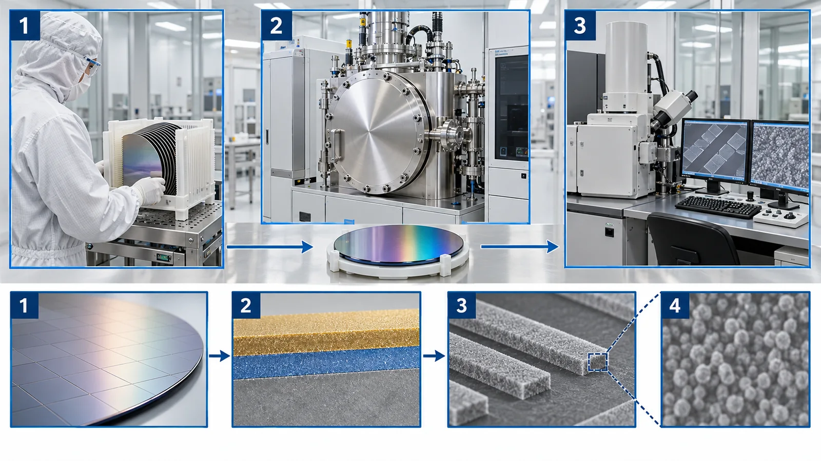
A laboratory changes materials and competes for the best single device. A foundry competes on making hundreds alike with the same process. As Van Damme and co-workers showed, the first step is to confirm that “more than 100 µs is obtained in wafer-wide statistics”; the next task can be read as moving material improvements such as tantalum and silicon substrates into industrial processes (our commentary; the paper does not say it will introduce tantalum next). From the materials side the job is to make new metals, substrates and cleaning steps compatible with the contamination control of a production line.
3. Materials of other approaches — silicon, diamond, ions, topological
In approaches other than superconducting ones too, “the quality of the material decides performance.” The review by de Leon and co-workers sums up the materials challenges of five approaches to quantum computing [Reference 7]. To connect with other articles in this series, the table gives only the materials points. For details, see each article.
| Approach | Main materials issues | What has been reported | For details |
|---|---|---|---|
| Silicon spin | Reduce nuclear-spin-carrying 29Si (isotope-purified 28Si). Quality of the interface between silicon and oxide or SiGe (valley splitting, charge noise) | In devices made on a 300 mm foundry line, all 4 devices had fidelity above 99% and state preparation and measurement reached up to 99.9% (Nature version) Sourced [34] | Our explainer on silicon spin qubits |
| Diamond (NV centers; for quantum sensing) | Reduce 13C (about 1.1% in nature). Amount and placement of nitrogen | In CVD diamond with 13C reduced to about 0.3%, T2 was 1.8 ms Sourced [35] | Our explainer on quantum sensing |
| Ion traps | Electric-field noise at the electrode surface (which heats the ions) | The review by Brownnutt and co-workers collects measurements of surface electric-field noise using ions [26]. Hite and co-workers cleaned in situ with an argon-ion beam and cut electric-field noise by a factor of 100 (as in the title) [27] Sourced | Our explainer on ion traps |
| Topological (Majorana) | Quality of the interface between semiconductor and superconductor; the hard gap | Chang and co-workers reported a hard gap in epitaxial InAs–Al nanowires [36] Sourced. Assessment of progress of the approach as a whole is left to another article | Our explainer on topological quantum computing |
| Photonic and neutral atom | Optical components, waveguides, vacuum quality and so on | Not covered here | Our explainers on photonic quantum computing and neutral atoms, among others |
Each number is as stated in the individual paper. They are not for ranking the approaches.
In superconducting qubits it is the oxide at surfaces and interfaces; in silicon and diamond, isotopes and nuclear spins; in ions, the electrode surface; in topological qubits, the interface between semiconductor and superconductor. The forms differ, but how the qubit touches the materials around it, and where decides performance (our summary). For a materials engineer, whichever approach wins, familiar skills such as surface analysis, isotope analysis and thin-film deposition have their place.
4. Cryogenic wiring and heat — the budget set by cooling power
The dilution refrigerator that cools qubits to between a few mK and 20 mK (see our explainer on cryogenics and control) has a severe upper limit on how much it can cool. On top of that, the wiring (coaxial cables) that drives the qubits carries heat from room temperature to the cold stages. For a materials engineer this means that the thermal conductivity of materials can directly set how large a quantum computer can be.
4.1 The refrigerator's “budget”
Fig. 10 shows the temperature and cooling power of each stage of the commercial dilution refrigerator (Bluefors XLD400) used in the paper by Krinner and co-workers. The lower the temperature, the cooling power becomes smaller by orders of magnitude. The cooling power of the lowest stage (the mixing chamber, MXC) is 19 µW at 20 mK (when 40 mW of heating is applied to the still) Sourced [Reference 23]. 19 µW is about one fifty-thousandth of 1 W Our calculation.
4.2 Heat from wiring — a simple calculation for a feel of the scale
Krinner and co-workers calculated that running 50 qubits needs 124 RF lines in total (50 drive, 50 flux, 8 output, 8 input, 8 amplifier pump). The heat load on the MXC is about 30% of that stage's cooling power (with passive heat and active heat from signal dissipation roughly equal), the operating temperature is about 14 mK, and if the capacity for coaxial cables could be tripled, 150 qubits could be operated Sourced [Reference 23].
Here is a simple division. Dividing the MXC's 19 µW (at 20 mK) by 124 lines gives about 0.15 µW per line (150 nW). With 1,000 lines it would be about 19 nW per line Our calculation (the cooling power is the value at 20 mK, whereas the paper's design is at 14 mK, and heat is not shared out line by line, so this is a rough calculation to get a feel for orders of magnitude). In other words, as qubits increase, the heat allowed per line shrinks rapidly. Krinner and co-workers also write that for about 1,000 qubits the design must be revisited: making the flux lines superconducting NbTi to remove active heat, tolerating a cold plate at about 200 mK (cooling power of at least 400 µW), and tolerating a base temperature of 30 mK (cooling power about 40 µW) [Reference 23].
Wiring is required to carry electrical signals well and carry as little heat as possible. Metals that conduct electricity well also conduct heat well, so this is a contradictory requirement. For the output lines, Krinner and co-workers chose stainless-steel (SS) coaxial cable between 4 K and room temperature and superconducting NbTi coaxial cable between the MXC and 4 K, and state that stainless-steel and NbTi coaxial cables have the lowest passive heat load [Reference 23]. Passive heat is set by integrating the thermal conductivity of the material over temperature (Eq. (1) of the paper). Published data on the thermal conductivity of materials can be found on NIST's cryogenic materials page and elsewhere [Reference 31]. Thinning the cable (0.085 inch to 0.047 inch) cuts passive heat to about a quarter, since it scales with the square of the diameter, but signal attenuation grows and DC resistance rises, so the active heat from flux biasing becomes about four times larger; this trade-off is also shown [Reference 23].
- Blocking infrared: infrared radiation creates quasiparticles and shortens T1. Krinner and co-workers describe the option of installing an infrared filter made of Eccosorb CR-124 absorber just before the attenuator at the MXC (6 dB attenuation at 6 GHz) [Reference 23]. It is an example of an absorbing material protecting a qubit's lifetime
- Supply of helium-3: dilution refrigerators use helium-3. In 2009 Science reported that a helium-3 shortage could freeze low-temperature research (as in the article's title) [Reference 30]. We have not, however, checked the later supply and price (Section 6)
Wrong: “just make the refrigerator bigger and more powerful.” In fact: cooling power becomes smaller by orders of magnitude at lower temperature (Fig. 10), and heat from wiring grows in proportion to the number of lines. Adding stages or enlarging the unit also changes the balance among cable length, thermal conduction of the materials and signal attenuation. As Krinner and co-workers do by examining cable materials, line counts and permitted temperatures of the cooling stages together, materials, wiring and refrigerator must be designed as a set (our commentary).
5. What limits performance — sorting out the factors
Here we sort what we have covered by the question “what is limiting performance?” There is no single culprit; the limiting factor changes with the stage a qubit has reached. The positioning below is this article's own summary based on what has been reported.
T1, Q, fidelity and so on are values for individual physical qubits. They are not the performance of a logical qubit built by error correction. As physical qubits improve, the number needed to build a logical qubit and the burden of error correction change (see our explainer on logical qubits and fault-tolerant quantum computing).
| Factor | Where it acts | Basis (source) | Positioning (our summary) |
|---|---|---|---|
| Amorphous oxide at surfaces and interfaces (TLS) | Superconducting qubits. Surfaces of metal and substrate | Loss is orders of magnitude above the bulk limit, with the cause in uncontrolled surfaces, interfaces and contaminants [1]. The nature of TLS is unresolved [10]. Nb oxide is especially lossy [4, 11, 12] Sourced | One of the present main causes. Countermeasures (capping, Ta, cleaning) have brought large gains |
| Bulk substrate loss | Superconducting qubits (Ta on sapphire) | Surface and bulk dielectric loss are comparable [3, 13]. High-resistivity silicon markedly lowered bulk loss [3] Sourced | A limit that emerges after the surface is dealt with. Improved by choice of substrate |
| Around the junction (parasitic junctions, junction quality) | Superconducting qubits | Parasitic junctions can cause dielectric loss [15]. Where T2 (echo) exceeds T1, junction-related decoherence began to be seen [3] Sourced | The limit that shows up next in long-lived devices |
| Junction spread | Many qubits | Frequency is proportional to Rn to the power −1/2 [17]. Collisions multiply when σf exceeds 30 MHz, and with 10 MHz a heavy-hex lattice is collision-free with probability about 92% (distance-5 lattice) [17]. Improved by laser tuning after fabrication [17] Sourced | A limit that sets the scale. A problem separate from the lifetime of one qubit |
| Quasiparticles, radiation, infrared | Superconducting qubits | Radiation limits today's type of qubit in the millisecond regime [19]. Breaks many qubits at once [20]. Burst frequency 1/50 underground [21] Sourced | A small effect today. A limit that matters at the fault-tolerant stage |
| Reproducibility on a production line | Superconducting (foundry) | imec: above 100 µs [16]. Google 105-qubit chip, mean T1: 68 µs [22]. Laboratory best: 0.5 to 1.7 ms [2, 3, 4, 5] Sourced | The gap between best and production values is the present challenge |
| Cooling and wiring heat | When the number of qubits increases | MXC cooling power is 19 µW (at 20 mK) [23]. 124 lines for 50 qubits [23] Sourced | A limit that sets the scale. Eased by wiring materials and design |
| Materials of other approaches | Silicon spin, diamond, ions, topological | The table in Section 3 | A different limit for each approach (isotopes, interfaces, electrode surfaces and so on) |
“Positioning” is this article's summary based on the statements of each paper; it does not mean the authors give the same ordering.
A small calculation: why surface and bulk are both needed
Loss is a sum (1/Q = Σ participation × loss tangent). Crowley and co-workers report that in Ta resonators the surface and bulk TLS contributions are comparable [Reference 13]. Suppose the surface loss (1/Qsurface) and the bulk loss (1/Qbulk) are exactly equal and there is no other loss. Then 1/Q = 2/Qsurface, so Q = Qsurface / 2. Even if the bulk loss were removed completely, Q would only double. To go further, the surface loss must also come down Our calculation (a simplified model of this article; real devices have other losses too). It points the same way as the conclusion of Crowley and co-workers, that improvements in both surface and bulk are needed.
When performance is poor, “the material is bad” is not a countermeasure. You need to separate which loss, at which place. For that, methods of measuring loss with resonators have been refined (the review by McRae and co-workers gives recommendations for designing loss measurements and reporting results [9]). Wang and co-workers showed the relation between the fraction of electric-field energy stored in the surface dielectric (the surface participation) and the relaxation rate, and used it to locate loss [14]. Altoé and co-workers pinned down where loss sits by selectively changing the interface dielectrics [11]. This is the same “separating the factors” approach used in developing semiconductor and battery materials (our commentary).
Wrong: “switch to tantalum and qubits will live long.” In fact: in Place and co-workers' Ta on sapphire, surface and bulk loss are comparable (as in the calculation above); Bland and co-workers replaced the substrate with high-resistivity silicon, and T1 reached up to 1.68 ms; then, with low-contamination junction deposition, T2 (echo) exceeded T1 [References 3, 1]. Bal and co-workers report that niobium covered with a Ta cap gave a median T1 above 300 µs (maximum 600 µs) [4]. It is not the name of a material but the combination of material, surface, substrate and process that decides the result (our summary).
6. What we could not confirm, and a summary
What we could not confirm
- Latest performance and yield on production lines: we checked the values of imec and Google, but IBM's blog (a company claim) gives no performance values, and we have not exhaustively checked other companies or values from 2026 onward [References 16, 22, 29].
- Examples of introducing new materials such as tantalum into a foundry production line: we could not confirm any.
- The microscopic nature of TLS: Müller and co-workers' review describes it as an unresolved question [Reference 10]. We have not exhaustively checked later progress.
- Reproduction of Bland et al.'s Ta on high-resistivity Si on larger chips or on a production line: not confirmed. What the paper has is a time-averaged Q of 9.7 × 10⁶ across 45 qubits and a statement that it could potentially be made at wafer scale [Reference 3].
- The latest supply and price of helium-3: we have only the title of a 2009 news report [Reference 30] and have not checked the current situation.
- Cooling power of newer dilution refrigerators: only the values for the one model of Krinner et al. [Reference 23].
- Standards specific to the materials and manufacture of qubits: we could not confirm any (Section 7).
- Materials issues of non-solid-state approaches such as photonic and neutral-atom, and research programmes and company efforts in Japan: not covered in this article.
- A large part of a qubit's performance is decided by surfaces, interfaces, defects, isotopes and heat in the materials. In superconducting qubits, amorphous oxide a few nanometres thick (TLS) is one of the leading sources of loss. Oxide where the electric field passes shortens the lifetime Sourced
- Countermeasures are advancing. Capping niobium, using tantalum, and putting the qubits on high-resistivity silicon. The best T1 has reached 1.68 ms. But both surface and bulk must be lowered (even in our calculation, treating only one gives at most a factor of two), so it is not a story solved by one material Sourced / Our calculation
- The “best single device” and “hundreds that match” are different contests. Between the laboratory best (0.5 to 1.7 ms) and values on 300 mm production lines or large chips (68 to just over 100 µs) there is a gap of more than a factor of ten. Matching junction resistance to within 1% is also needed to avoid frequency collisions Sourced / Our calculation
- There are limits that come from outside the material, too. Radiation limits today's type of qubit in the millisecond regime. A refrigerator's cooling power is smaller by orders of magnitude at lower temperature, and the heat from wiring limits the number of qubits Sourced
- The same viewpoint works in other approaches. Isotopes in silicon spin, 13C in diamond, electrode surfaces for ions, interfaces in topological qubits. A materials engineer's knowledge of surface analysis, thin-film deposition, isotope analysis and thermal design connects directly to a quantum computer's performance (our summary)
7. How to read evaluations and standards
The performance of materials and manufacturing is measured by the internal Q and loss tangent of resonators, the T1 and T2 of qubits, junction spread (σ), yield, and cooling power and heat load. No single number tells you enough. On the standards side, an international standard for the vocabulary of quantum computing has been published, but a dedicated standard for measuring material loss or manufacturing quality could not be confirmed within the scope of our survey.
| Item | Representative benchmarks and methods (name, source) | Standards and guidance (ISO/IEC, IEEE and so on) | Cautions in reading |
|---|---|---|---|
| Material loss (resonators) | Internal Q, loss tangent tanδ, participation (the surface participation of Wang et al., 2015). The review of McRae et al. (2020) gives the design of measurements and recommendations for reporting [9, 14] Sourced | Could not be confirmed | Values change with single-photon power, temperature and device shape. Check that the reporting format is common |
| Qubit coherence | T1, T2 (echo). How they are measured and whether average or best differ by report [1 to 5] (see our explainer on coherence and fidelity) | Could not be confirmed (whether ISO/IEC 4879 includes coherence terms is unverified) | For the same Q, a lower frequency gives a longer T1 (the calculation in Section 2.4). Always check mean or median versus best |
| Junction spread | Relative standard deviation of critical current and resistance (σR, σIc), and standard deviation of frequency σf (Kreikebaum, Osman, Hertzberg) [15, 17, 18] Sourced | Could not be confirmed | Depends on within-chip versus whole-wafer and on junction size. The same “%” cannot be compared |
| Production statistics | Wafer-wide coherence, yield, variability and ageing (imec) [16] Sourced | Semiconductor standards fall under IEC/TC 47 and are outside JTC 3 (below). A SEMI standard specific to qubits could not be confirmed | Whether the format of industrial standards can be used as is for qubits is unverified |
| Cooling power and heat load | Specification of “cooling power at each temperature” (W at K) for each stage, passive and active heat from wiring (Krinner et al.) [23] Sourced. Published thermal-conductivity data for materials (NIST) [31] | Cryogenic vessels fall under ISO/TC 220 and are outside JTC 3 (below) | Cooling power differs by orders of magnitude with temperature. Always check the temperature given with a “cooling power.” Only one model |
| Terminology and scope | — (a standard for terms and scope, not an evaluation) | ISO/IEC 4879:2024 “Information technology — Quantum computing — Vocabulary” (published May 2024, edition 1, 14 pages, published) [32]. The scope of IEC/ISO JTC 3 includes quantum information (quantum computing and simulation), quantum metrology and quantum detectors. Excluded: semiconductors (IEC/TC 47), cryogenic vessels (ISO/TC 220), fibre optics (IEC/TC 86), nanotechnology (IEC/TC 113 and ISO/TC 229). One standard published, 12 under development [33]. JTC 3 has liaison with IEC/TC 90 (Superconductivity) and others [33] Sourced | The text of the standards is paid and we have not checked it. IEEE P7130 (Quantum Technologies Definitions) is a draft [37]; this time we could not access the IEEE page and have not re-checked its status Not yet confirmed |
The table is our summary (Our calculation). Numbers are reference numbers. Numbers, titles and status of standards were checked on the official ISO pages (checked 16 October 2026). Because the text of standards is paid, we limit ourselves to titles and scope.
Cautions in reading (for materials engineers)
- Best values and values that match are different: the T1 of 1.68 ms is the maximum for one device, and 68 µs is the average of a 105-qubit chip. They differ by more than a factor of ten, which is the core of this article [3, 22]
- T1 depends on frequency: to compare materials, look at Q or the loss tangent. Values at different frequencies, photon numbers and temperatures cannot be compared as they stand [9]
- A company announcement is a company claim: announcements with no performance values, or introductions of a company's own manufacturing, like IBM's blog, are not treated as fact until they can be checked against primary sources (papers) [29]
- Note what is “not there” in standards: we could not confirm a dedicated standard for measuring material loss or manufacturing quality. Because there is none, the reader has to check each paper's measurement method and reporting format. Semiconductors, cryogenic vessels and superconductivity each fall under separate standards bodies [33]
- Plans and achievements are different: a draft such as IEEE P7130 is Not yet confirmed. IBM's roadmap and future chips on 300 mm are also plans
8. Glossary
- Physical qubit / logical qubit
- A physical qubit is a single actual device. A logical qubit is made by bundling many physical qubits for error correction. All numbers in this article are for physical qubits.
- Josephson junction
- A structure with a very thin insulating film between two superconductors. It acts as a non-linear inductor.
- Transmon
- The representative type of superconducting qubit, made from a Josephson junction and a capacitor.
- T1
- The time for a qubit to lose energy and return to its ground state (its lifetime).
- T2 (echo)
- The time over which phase information is kept. Measured by the Hahn-echo method, which cancels slow noise.
- Q (quality factor)
- The sharpness of a resonance. The larger Q is, the smaller the loss. T1 = Q ÷ (2π f).
- Loss tangent (tanδ)
- A property of a material that expresses the rate at which a dielectric loses energy.
- Participation
- The fraction of the electric-field energy stored in a given place (for example, a surface oxide).
- TLS (two-level system)
- A small defect in an amorphous material that can switch between two states. It takes energy from a qubit.
- Amorphous
- A state in which atoms are not arranged regularly as in a crystal. Native oxide films are mostly amorphous.
- Cooper pair
- A pair of electrons bound together in a superconductor. It flows without resistance.
- Quasiparticle
- An excitation that appears when a Cooper pair breaks. It takes energy from a qubit.
- Native oxide
- An oxide film that forms naturally on a metal surface on contact with air.
- Passivation (capping)
- Covering a surface with another material to prevent oxidation and the like.
- Angled (shadow) evaporation
- Evaporating metal from an oblique direction and using the shadow of the resist to make an overlap.
- Lift-off
- A step that dissolves the resist, and the excess metal on it, away.
- RIE (reactive-ion etching)
- Etching a material with ions of reactive gases. A standard method on foundry lines.
- Parasitic junction
- A structure like a Josephson junction that arises unintentionally. It can cause dielectric loss.
- Frequency collision
- When the frequencies of neighbouring qubits are in a relation that increases gate errors.
- Relative standard deviation
- Spread expressed as a fraction of the mean.
- Yield
- The fraction of what is made that is usable.
- CMOS pilot line / foundry
- A trial line for the processes used in semiconductor volume production / a contract-manufacturing factory.
- High-resistivity silicon
- Silicon with few impurities and very high electrical resistance. Used as a substrate with low microwave loss.
- 28Si (isotope purification)
- Silicon with nuclear-spin-carrying 29Si reduced. It lowers the noise of silicon spin qubits.
- Hard gap
- A state in which there are almost no extra states inside the superconducting gap.
- Dilution refrigerator
- A device that cools to millikelvin temperatures using a mixture of helium-3 and helium-4.
- MXC (mixing chamber)
- The coldest stage of a dilution refrigerator. The qubits sit here.
- NbTi
- An alloy of niobium and titanium. It becomes superconducting at low temperature and conducts little heat, so it is used for cryogenic wiring.
- Thermal conductivity
- How easily a material conducts heat. In wiring material selection it pulls against ease of conducting electricity.
9. References (primary sources)
- Place A. P. M. et al. "New material platform for superconducting transmon qubits with coherence times exceeding 0.3 milliseconds", Nature Communications 12, 1779 (2021), DOI 10.1038/s41467-021-22030-5 — doi.org/10.1038/s41467-021-22030-5
- Wang C. et al. "Towards practical quantum computers: transmon qubit with a lifetime approaching 0.5 milliseconds", npj Quantum Information 8, 3 (2022), DOI 10.1038/s41534-021-00510-2 — doi.org/10.1038/s41534-021-00510-2
- Bland M. P. et al. "Millisecond lifetimes and coherence times in 2D transmon qubits", Nature 647, 343–348 (2025), DOI 10.1038/s41586-025-09687-4 (arXiv:2503.14798) — doi.org/10.1038/s41586-025-09687-4
- Bal M. et al. "Systematic improvements in transmon qubit coherence enabled by niobium surface encapsulation", npj Quantum Information 10, 43 (2024), DOI 10.1038/s41534-024-00840-x (arXiv:2304.13257) — doi.org/10.1038/s41534-024-00840-x
- Tuokkola M. et al. "Methods to achieve near-millisecond energy relaxation and dephasing times for a superconducting transmon qubit", Nature Communications 16, 5421 (2025), DOI 10.1038/s41467-025-61126-0 (arXiv:2407.18778) — doi.org/10.1038/s41467-025-61126-0
- Siddiqi I. "Engineering high-coherence superconducting qubits", Nature Reviews Materials 6, 875–891 (2021), DOI 10.1038/s41578-021-00370-4 — doi.org/10.1038/s41578-021-00370-4
- de Leon N. P. et al. "Materials challenges and opportunities for quantum computing hardware", Science 372, eabb2823 (2021), DOI 10.1126/science.abb2823 — doi.org/10.1126/science.abb2823
- Oliver W. D., Welander P. B. "Materials in superconducting quantum bits", MRS Bulletin 38, 816–825 (2013), DOI 10.1557/mrs.2013.229 — doi.org/10.1557/mrs.2013.229
- McRae C. R. H. et al. "Materials loss measurements using superconducting microwave resonators", Rev. Sci. Instrum. 91, 091101 (2020), DOI 10.1063/5.0017378 (arXiv:2006.04718) — doi.org/10.1063/5.0017378
- Müller C., Cole J. H., Lisenfeld J. "Towards understanding two-level-systems in amorphous solids: insights from quantum circuits", Rep. Prog. Phys. 82, 124501 (2019), DOI 10.1088/1361-6633/ab3a7e — doi.org/10.1088/1361-6633/ab3a7e
- Altoé M. V. P. et al. "Localization and mitigation of loss in niobium superconducting circuits", PRX Quantum 3, 020312 (2022), DOI 10.1103/PRXQuantum.3.020312 (arXiv:2012.07604) — doi.org/10.1103/PRXQuantum.3.020312
- Verjauw J. et al. "Investigation of microwave loss induced by oxide regrowth in high-Q Nb resonators", Phys. Rev. Applied 16, 014018 (2021), DOI 10.1103/PhysRevApplied.16.014018 (arXiv:2012.10761) — doi.org/10.1103/PhysRevApplied.16.014018
- Crowley K. D. et al. "Disentangling losses in tantalum superconducting circuits", Phys. Rev. X 13, 041005 (2023), DOI 10.1103/PhysRevX.13.041005 (arXiv:2301.07848) — doi.org/10.1103/PhysRevX.13.041005
- Wang C. et al. "Surface participation and dielectric loss in superconducting qubits", Appl. Phys. Lett. 107, 162601 (2015), DOI 10.1063/1.4934486 — doi.org/10.1063/1.4934486
- Osman A. et al. "Simplified Josephson-junction fabrication process for reproducibly high-performance superconducting qubits", Appl. Phys. Lett. 118, 064002 (2021), DOI 10.1063/5.0037093 (arXiv:2011.05230) — doi.org/10.1063/5.0037093
- Van Damme J. et al. "Advanced CMOS manufacturing of superconducting qubits on 300 mm wafers", Nature 634, 74–79 (2024), DOI 10.1038/s41586-024-07941-9 — doi.org/10.1038/s41586-024-07941-9
- Hertzberg J. B. et al. "Laser-annealing Josephson junctions for yielding scaled-up superconducting quantum processors", npj Quantum Information 7, 129 (2021), DOI 10.1038/s41534-021-00464-5 (arXiv:2009.00781) — doi.org/10.1038/s41534-021-00464-5
- Kreikebaum J. M., O'Brien K. P., Morvan A., Siddiqi I. "Improving wafer-scale Josephson junction resistance variation in superconducting quantum coherent circuits", Supercond. Sci. Technol. 33, 06LT02 (2020), DOI 10.1088/1361-6668/ab8617 (arXiv:1909.09165) — doi.org/10.1088/1361-6668/ab8617
- Vepsäläinen A. P. et al. "Impact of ionizing radiation on superconducting qubit coherence", Nature 584, 551–556 (2020), DOI 10.1038/s41586-020-2619-8 (arXiv:2001.09190) — doi.org/10.1038/s41586-020-2619-8
- McEwen M. et al. "Resolving catastrophic error bursts from cosmic rays in large arrays of superconducting qubits", Nature Physics 18, 107–111 (2022), DOI 10.1038/s41567-021-01432-8 (arXiv:2104.05219) — doi.org/10.1038/s41567-021-01432-8
- Cardani L. et al. "Reducing the impact of radioactivity on quantum circuits in a deep-underground facility", Nature Communications 12, 2733 (2021), DOI 10.1038/s41467-021-23032-z (arXiv:2005.02286) — doi.org/10.1038/s41467-021-23032-z
- Google Quantum AI "Quantum error correction below the surface code threshold", Nature 638, 920–926 (2025), DOI 10.1038/s41586-024-08449-y (arXiv:2408.13687) — doi.org/10.1038/s41586-024-08449-y
- Krinner S. et al. "Engineering cryogenic setups for 100-qubit scale superconducting circuit systems", EPJ Quantum Technology 6, 2 (2019), DOI 10.1140/epjqt/s40507-019-0072-0 (arXiv:1806.07862) — doi.org/10.1140/epjqt/s40507-019-0072-0
- Dolan G. J. "Offset masks for lift-off photoprocessing", Appl. Phys. Lett. 31, 337–339 (1977), DOI 10.1063/1.89690 — doi.org/10.1063/1.89690
- Lecocq F. et al. "Junction fabrication by shadow evaporation without a suspended bridge", Nanotechnology 22, 315302 (2011), DOI 10.1088/0957-4484/22/31/315302 — doi.org/10.1088/0957-4484/22/31/315302
- Brownnutt M. et al. "Ion-trap measurements of electric-field noise near surfaces", Rev. Mod. Phys. 87, 1419–1482 (2015), DOI 10.1103/RevModPhys.87.1419 — doi.org/10.1103/RevModPhys.87.1419
- Hite D. A. et al. "100-fold reduction of electric-field noise in an ion trap cleaned with in situ argon-ion-beam bombardment", Phys. Rev. Lett. 109, 103001 (2012), DOI 10.1103/PhysRevLett.109.103001 — doi.org/10.1103/PhysRevLett.109.103001
- Kjaergaard M. et al. "Superconducting qubits: current state of play", Annu. Rev. Condens. Matter Phys. 11, 369–395 (2020), DOI 10.1146/annurev-conmatphys-031119-050605 — doi.org/10.1146/annurev-conmatphys-031119-050605
- IBM Quantum (company technical blog) "Building quantum computers with leading-edge semiconductor fab (dated 12 November 2025)", IBM Quantum Computing Blog (company claim) — www.ibm.com/quantum/blog/300mm-fab
- Cho A. "Helium-3 shortage could put freeze on low-temperature research (title cited only)", Science 326, 778–779 (2009), DOI 10.1126/science.326_778 — doi.org/10.1126/science.326_778
- NIST "Cryogenic Material Properties (page of cryogenic material property data)", NIST Cryogenic Technologies Group — trc.nist.gov/cryogenics/materials/materialproperties.htm
- ISO/IEC "ISO/IEC 4879:2024 Information technology — Quantum computing — Vocabulary (ISO page)", ISO — committee.iso.org/standard/80432.html
- ISO/IEC "IEC/ISO JTC 3 Quantum technologies (committee page)", ISO — committee.iso.org/committee/10138914.html
- Steinacker P., Dumoulin Stuyck N. et al. "Industry-compatible silicon spin-qubit unit cells exceeding 99% fidelity", Nature 646, 81–87 (2025), DOI 10.1038/s41586-025-09531-9 — doi.org/10.1038/s41586-025-09531-9
- Balasubramanian G. et al. "Ultralong spin coherence time in isotopically engineered diamond", Nature Materials 8, 383–387 (2009), DOI 10.1038/nmat2420 — doi.org/10.1038/nmat2420
- Chang W. et al. "Hard gap in epitaxial semiconductor–superconductor nanowires", Nature Nanotechnology 10, 232–236 (2015), DOI 10.1038/nnano.2014.306 — doi.org/10.1038/nnano.2014.306
- IEEE SA "IEEE P7130 Standard for Quantum Technologies Definitions (draft)", IEEE SA (the page could not be accessed this time and its status was not re-checked) — standards.ieee.org/ieee/7130/10680/
10. Claim-to-source audit
| Claim in the article | Primary source (where it appears) | Type |
|---|---|---|
| The junction is Al / AlOx / Al. The transmon is an anharmonic oscillator made of a non-linear inductor (the Josephson junction) with a capacitor. Angled evaporation (Dolan 1977), the bridge-free (Manhattan-style) method, dynamic oxidation, and patch integration in one vacuum cycle (PICT) | Abstracts and text of Kreikebaum et al. (2020), Osman et al. (2021), Dolan (1977) and Lecocq et al. (2011) Reference 18 https://doi.org/10.1088/1361-6668/ab8617 Reference 15 https://doi.org/10.1063/5.0037093 Reference 24 https://doi.org/10.1063/1.89690 Reference 25 https://doi.org/10.1088/0957-4484/22/31/315302 | Sourced |
| Transmons are weakly anharmonic, with transition energies that fall at higher levels. f scales roughly as R_n to the power -1/2. sigma_f 132.3 MHz (2.3%), sigma_R 4.6%, after laser tuning sigma_R 0.61% and sigma_f 14.0 MHz (9.5-fold improvement). Collision window +/-17 MHz. At sigma_f = 10 MHz, heavy-hex 92% and square lattice 0.8% collision-free (distance 5); above 30 MHz, more than 10 collisions | Abstract, text and Table I of Hertzberg et al. (2021) Reference 17 https://doi.org/10.1038/s41534-021-00464-5 | Sourced |
| 150 mm wafer, 64 chips of 1 x 1 cm, room-temperature resistance +/-30%. For 3,000 junctions over 49 cm2, relative standard deviation of critical current below 3.5%; mean 1.8% within 1 x 1 cm (some below 1.0%). A study of 38 wafers | Abstract of Kreikebaum et al. (2020) Reference 18 https://doi.org/10.1088/1361-6668/ab8617 | Sourced |
| More than 3,600 junctions; 3.7% across the wafer, 2.7% mean within a chip (20 chips at 1.4 to 2%). Frequency variation 1.7 to 2.5%, of which 60 to 70% is junction-area fluctuation. Mean T1 above 50 us (Q > 1.5 x 10^6). Parasitic junctions contribute to dielectric loss. Earlier reports such as 10 to 20% (Lotkhov et al., Al junctions of 0.125 to 0.25 um2) | Abstract and introduction of Osman et al. (2021) Reference 15 https://doi.org/10.1063/5.0037093 | Sourced |
| Relaxation times orders of magnitude shorter than the bulk limit; cause in uncontrolled surfaces, interfaces and contaminants. Ta gives above 0.3 ms, increased in 17 devices (sapphire substrate) | Abstract of Place et al. (2021) Reference 1 https://doi.org/10.1038/s41467-021-22030-5 | Sourced |
| Dry etching of Ta gives best T1 of 503 us. Comparison of Ta, Nb and Al gives Ta > Al > Nb. The difference is attributed to oxide loss at the metal-air interface | Abstract of Wang et al. (2022) Reference 2 https://doi.org/10.1038/s41534-021-00510-2 | Sourced |
| In-situ capping of the Nb surface (Ta, Al, TiN, Au). T1 2 to 5 times longer. With a Ta cap, median above 300 us and maximum 600 us (sapphire and silicon). Nb oxide is more harmful than the native oxides of Ta, Al and TiN | Abstract of Bal et al. (2024) Reference 4 https://doi.org/10.1038/s41534-024-00840-x | Sourced |
| Median T1 425 us, maximum 666 +/- 33 us, median echo dephasing 541 us, maximum 1057 +/- 138 us, frequency 2.9 GHz. Design, fabrication and measurement setup reported in detail | Abstract of Tuokkola et al. (2025) Reference 5 https://doi.org/10.1038/s41467-025-61126-0 | Sourced |
| Ta on high-resistivity Si. Time-averaged Q of 9.7 x 10^6 across 45 qubits. Best device: time-averaged 1.5 x 10^7, maximum 2.5 x 10^7, T1 up to 1.68 ms. T2E exceeds T1. Single-qubit gate 99.994%. Potentially fabricable at wafer scale. Ta on sapphire is TLS-dominated, with comparable surface and bulk contributions | Abstract of Bland et al. (2025) (Nature version) Reference 3 https://doi.org/10.1038/s41586-025-09687-4 | Sourced |
| Internal Q of Ta resonators 5 to 15 x 10^6. Surface and bulk TLS contributions are comparable. Surface TLS can be altered by chemical processing | Abstract of Crowley et al. (2023) Reference 13 https://doi.org/10.1103/PhysRevX.13.041005 | Sourced |
| Nb resonators: HF removes the native oxide; with 16 minutes of exposure loss falls by an order of magnitude and single-photon internal Q reaches up to 7 x 10^6. The only oxide that grows significantly in the first 200 hours is Nb2O5. Loss is proportional to Nb2O5 thickness. tan delta = 9.9 x 10^-3 | Abstract of Verjauw et al. (2021) Reference 12 https://doi.org/10.1103/PhysRevApplied.16.014018 | Sourced |
| Most TLS loss comes from the silicon surface oxide and most non-TLS loss from the Nb surface oxide. Interface modification cut TLS loss by 85% and non-TLS loss by 72%. Single-photon Q above 5 million | Abstract of Altoé et al. (2022) Reference 11 https://doi.org/10.1103/PRXQuantum.3.020312 | Sourced |
| Reviews: the unresolved question of the nature of TLS. Recommendations for measuring and reporting material loss. Going from bulk to device introduces amorphous films and non-equilibrium excitations. Materials challenges of five approaches | Müller et al. (2019), McRae et al. (2020), Siddiqi (2021), de Leon et al. (2021), Oliver and Welander (2013), Kjaergaard et al. (2020) Reference 10 https://doi.org/10.1088/1361-6633/ab3a7e Reference 9 https://doi.org/10.1063/5.0017378 Reference 6 https://doi.org/10.1038/s41578-021-00370-4 Reference 7 https://doi.org/10.1126/science.abb2823 Reference 8 https://doi.org/10.1557/mrs.2013.229 Reference 28 https://doi.org/10.1146/annurev-conmatphys-031119-050605 | Sourced |
| Loss is roughly proportional to the participation of the surface dielectric layers (surface participation) | Wang et al. (2015) Reference 14 https://doi.org/10.1063/1.4934486 | Sourced |
| Environmental radiation raises quasiparticle density and limits T1 of today's type of qubit to the millisecond regime. Shielding tends to lengthen coherence. Earlier reports that infrared photons increase quasiparticles. The effect of radiation is small in today's qubits | Abstract of Vepäläinen et al. (2020) Reference 19 https://doi.org/10.1038/s41586-020-2619-8 | Sourced |
| A particle impact ionises the substrate; bursts of phonons and quasiparticles simultaneously limit the energy coherence of all qubits, causing chip-wide failure | Abstract of McEwen et al. (2021) Reference 20 https://doi.org/10.1038/s41567-021-01432-8 | Sourced |
| In a deep-underground lead-shielded cryostat, burst frequency fell by a factor of 50 and dissipation by up to a factor of 4 | Abstract of Cardani et al. (2021) Reference 21 https://doi.org/10.1038/s41467-021-23032-z | Sourced |
| On a 300 mm CMOS pilot line, using only optical lithography and RIE, T1 and T2 above 100 us. Wafer-wide statistics (coherence, yield, variability, ageing). In line with laboratory methods. Potential for three-dimensional integration. Industrial processes were not optimised for high coherence and not a priori compatible with the usual methods | Abstract of Van Damme et al. (2024) Reference 16 https://doi.org/10.1038/s41586-024-07941-9 | Sourced |
| 105-qubit processor. Mean T1 68 us and T2 (CPMG) 89 us of the qubits. Attributed to improved fabrication techniques, participation-ratio engineering and optimisation of circuit parameters | Text of Google Quantum AI (2025) (arXiv version) Reference 22 https://doi.org/10.1038/s41586-024-08449-y | Sourced |
| Loon, Nighthawk and future chips are made with 300 mm wafer technology at the Albany NanoTech Complex. Some wafers are cored to 200 mm for additional steps. No performance values given. Dated 12 November 2025 | IBM blog (company claim) Reference 29 https://www.ibm.com/quantum/blog/300mm-fab | Sourced (as a company claim) |
| Each stage of the dilution refrigerator (Bluefors XLD400): 35 K, 30 W (at 45 K); 2.85 K, 1.5 W (at 4.2 K); 0.88 K, 40 mW (at 1.2 K); 82 mK, 200 uW (at 140 mK); 6 mK, 19 uW (at 20 mK). 50 qubits and 124 lines, MXC load about 30% at 14 mK. 150 qubits if cable capacity is tripled. Revisions for 1,000 qubits (NbTi flux lines, CP about 200 mK at 400 uW, base 30 mK at about 40 uW). Cable-diameter trade-off; Eccosorb infrared filter (6 dB at 6 GHz) | Table 1 and text of Krinner et al. (2019) Reference 23 https://doi.org/10.1140/epjqt/s40507-019-0072-0 | Sourced |
| A news report on a helium-3 shortage (title only). A page of cryogenic material property data | Title of Cho (2009); NIST page Reference 30 https://doi.org/10.1126/science.326_778 Reference 31 https://trc.nist.gov/cryogenics/materials/materialproperties.htm | Sourced |
| Silicon spin: all 4 devices above 99% fidelity on a 300 mm foundry line, SPAM up to 99.9%. Diamond: 13C reduced to about 0.3% gives T2 of 1.8 ms. Ions: a 100-fold reduction in electric-field noise by in-situ cleaning (title). A hard gap in InAs / Al nanowires | Steinacker et al. (2025), Balasubramanian et al. (2009), Brownnutt et al. (2015), Hite et al. (2012), Chang et al. (2015) Reference 34 https://doi.org/10.1038/s41586-025-09531-9 Reference 35 https://doi.org/10.1038/nmat2420 Reference 26 https://doi.org/10.1103/RevModPhys.87.1419 Reference 27 https://doi.org/10.1103/PhysRevLett.109.103001 Reference 36 https://doi.org/10.1038/nnano.2014.306 | Sourced |
| ISO/IEC 4879:2024 (vocabulary of quantum computing, May 2024, edition 1, 14 pages). The scope of JTC 3 and its exclusions (IT: JTC 1; nanotechnology: TC 113 and TC 229; fibre optics: TC 86; cryogenic vessels: TC 220; semiconductors: TC 47). One standard published, 12 under development. Liaison with IEC/TC 90 and others. IEEE P7130 is a draft | ISO pages (checked 16 October 2026). The IEEE page could not be accessed this time Reference 32 https://committee.iso.org/standard/80432.html Reference 33 https://committee.iso.org/committee/10138914.html Reference 37 https://standards.ieee.org/ieee/7130/10680/ | Sourced / Not yet confirmed |
| The example 1/Q = sum of participation x loss tangent (participation 10^-4 x 9.9 x 10^-3 gives Q of about 10^6, about 32 us at 5 GHz); conversion from Q to T1 (at 5 GHz: about 32 us for 10^6, about 320 us for 10^7, about 0.8 ms for 2.5 x 10^7); the frequency back-calculated from Bland et al.'s maximum Q and maximum T1 (about 2.4 GHz); at 5.43 GHz a 1% resistance shift gives about 27 MHz; the rough division of the MXC's 19 uW by 124 and by 1,000 lines (about 0.15 uW and about 19 nW); 30 W / 19 uW = about 1.6 x 10^6; 19 uW is about one fifty-thousandth of 1 W; with equal surface and bulk contributions, removing one gives at most a doubling of Q | Our own calculation (uses the numbers of the sources; assumed values and assumptions are stated) (this article; our own) | Our calculation |
| The analogies of a bell's ring-down, the rungs of a ladder and piano strings; the materials readings (A materials engineer's view 1 to 6); the idea of losses adding up; the sorting of factors (main cause, next limit, limit that sets the scale) | This article's own summary and commentary based on published content. Not the views stated by each researcher (this article; our own) | Commentary |
| The latest performance and yield on production lines, introduction of new materials (such as Ta) into production lines, the latest progress on the nature of TLS, reproduction of Bland et al.'s method on larger chips, the latest supply of helium-3, cooling power of new models, standards specific to qubit materials and manufacturing, materials of non-solid-state approaches, efforts in Japan | Not stated, because it could not be confirmed in the primary sources reachable within our survey (this article; our own) | Commentary |
| That Figs. 2, 3, 4, 5 and 8 are explanatory drawings, that Figs. 6, 7 and 10 are drawings summarising reported values, and that Figs. 1 and 9 are ImageGen-generated conceptual illustrations | Note by this article (this article; our own) | Commentary |
Last updated: 16 October 2026. Sources are limited to primary ones (peer-reviewed papers, reviews, arXiv papers, IBM's technical blog (a company claim), and the official pages of ISO and NIST). Values such as T1 differ in qubit frequency, design and measurement method, and do not indicate superiority. Where a worked example uses an assumed value or assumption, the text says so. We could not confirm, and so do not state, the latest performance on production lines, the introduction of new materials into production, standards specific to the materials and manufacture of qubits, or the latest status of IEEE P7130. All figures are explanatory concept diagrams or drawings of reported values; Figs. 1 and 9 are ImageGen-generated conceptual illustrations.