TECHNOLOGY EXPLAINER
Photonic Quantum Computers
― How a photon becomes a qubit, the biggest wall of "optical loss," and the optical materials behind it
A photonic quantum computer uses particles of light (photons) as qubits. Photons are little affected by their environment and are easy to link by optical fiber, but photons normally pass through one another without interacting, so two-qubit gates need ingenuity. A photon also keeps travelling and is finally detected and gone, so it is handled differently from a "qubit that stays put." And the biggest challenge is that photons are lost a little at every component they pass (loss). This article explains, step by step with figures and small numerical examples: (1) how a photon becomes 0 and 1, (2) how to "connect" photons that pass through each other, (3) fusion-based quantum computation and the continuous-variable approach that measures the light wave, (4) why optical loss is decisive, (5) chip materials and temperature (cooling of detectors), and (6) the state of play as of the check date (16 October 2026) together with claims of quantum advantage and the rebuttals. Thin-film lithium niobate, silicon nitride waveguides, silicon photonics and photodetectors are covered in separate explainers in this series.
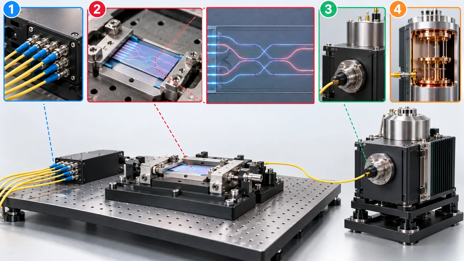
- In three lines / what to know first / where this sits in the series
- Recap: a qubit is an "arrow"
- How a photon becomes a qubit
- Photons pass through each other: so how do we "connect" them?
- Fusion-based quantum computation, and the continuous-variable approach
- The biggest wall: photon loss
- The key points on a common "card," and a side-by-side with the other three approaches
- Chips, materials and temperature
- Where things stand (checked 16 October 2026), plans, and claims of quantum advantage
- Limits, what we could not confirm, and a summary
- How to read evaluations and standards
- Glossary
- References (primary sources)
- Claim-to-source audit
Sourced = stated in a published source (with a link)
Our calculation = a value this article computed from stated assumptions
Not yet confirmed = plans, targets, drafts and other items that are not settled
Readings for materials research and analogies are marked as commentary. An inference is shown in bold.
A quantum-computing number means little unless it comes with what was measured and how. Here, error rates, fidelities and lifetimes come with the approach, the thing measured, whether it is an average or a best value, and the date. Company announcements are labeled as the company's claims, and plans and targets are shown as Not yet confirmed, kept apart from achieved facts. The loss graph in Chapter 6 is our own "feel-for-the-size" calculation, not an estimate of the loss of any real machine. We did not read the full texts of the standards (ISO/IEC, IEEE), which are paid; we give only titles and status. We do not tell lies to keep things simple. Every analogy comes with its limits.
1. In three lines / what to know first / where this sits in the series
- The qubit of a photonic quantum computer is a photon, a particle of light. For example, which of two waveguides (paths for light) holds the photon sets 0 and 1 (dual-rail). Photons are little affected by the environment (low decoherence), most parts can run at room temperature, and optical fiber can link them[Ref. 1, 2, 3]Sourced
- Photons pass through one another without interacting, so two-qubit gates are built with interference and measurement (the KLM scheme). Success is probabilistic, so fusion-based quantum computation, which combines small resource states with measurements called "fusions," is now a leading approach[Ref. 4, 5]Sourced
- The biggest challenge is photon loss. A little is lost at each component and it accumulates. Aghaee Rad et al. call optical loss "the dominant and most challenging hurdle" to crossing the fault-tolerant threshold[Ref. 2]Sourced. As of the check date, we could not confirm a report that achieved practical-scale error correction including loss
A photonic quantum computer "manipulates ever-travelling photons with interference and measurement." Its strengths are robustness to the environment and ease of linking by optical fiber. Its biggest challenge is that small losses at each component add up.
Prerequisites: none. The arrow picture is recapped in the next chapter (no quantum-mechanics formulas are used).
Place in the series: read this after "The Basics of Quantum Computing" and "Quantum Gates and Circuits." It is easiest to read side by side with the other three approaches (superconducting, trapped ions, neutral atoms). The materials behind photonic quantum computers are covered in our explainers on thin-film lithium niobate, silicon nitride waveguides, silicon photonics, photodetectors, semiconductor lasers and optical fiber. How to read claims of quantum advantage is in our explainer on that topic, and communication in our explainers on quantum key distribution and quantum communication, and on quantum networks and repeaters.
2. Recap: a qubit is an "arrow"
In this series, a qubit's state is drawn as an arrow from the center of a sphere to its surface. Pointing at the north pole means "0," pointing at the south pole means "1," and pointing in between is a superposition. When the arrow is tilted, a measurement always gives 0 or 1, and the chance of each is set by the tilt. After the measurement the arrow is fixed at a pole, and the old tilt does not come back.
That is wrong. A tilted arrow is not "holding both 0 and 1" but "pointing in a definite direction between 0 and 1." Measure it and you get just one of 0 or 1. A quantum computer's power comes from combining these arrow directions like waves so that the right answer reinforces itself (see our explainer on quantum algorithms).
3. How a photon becomes a qubit
Light is a wave and also a collection of "particles of light (photons)" (a property of the quantum world). A photonic quantum computer takes one photon as a qubit. The easiest encoding to picture is dual-rail. Two paths for light (waveguides) are placed side by side, and a photon in the upper waveguide is 0, in the lower one 1. When a photon goes through a half-silvered mirror (a beam splitter), it ends up "spread over both" paths. This is a superposition, the arrow tilted. Measured, it is found on just one path[Ref. 3, 6]Sourced. Combining beam splitters with phase shifters, which shift the phase of light, turns the arrow to any direction (one-qubit gates).
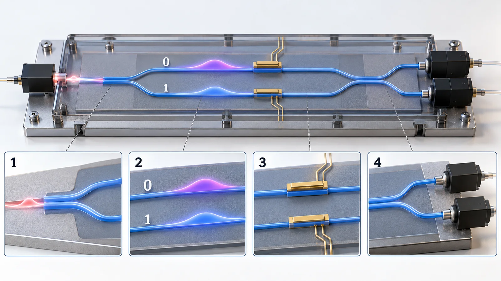
View original SVG, values and sources
Original SVG reference: Concept diagram (vector drawing). Concept diagram of dual-rail encoding of a photon and other ways to take 0 and 1 (polarization, time-bin). The encodings follow the review by Kok et al. [Ref. 3] and PsiQuantum's dual-rail qubits [Ref. 6].
Superconducting circuits and ions or atoms in vacuum are qubits that stay put in a chip or machine. A photon keeps travelling at the speed of light, so it is operated on as it passes through the chip and finally is caught by a detector and gone. So in a photonic quantum computer, rather than "placing a qubit in one spot and operating on it many times," computation means "applying operations one after another to the photons as they flow, and measuring at the end" (commentary). Limits of the analogy: "sorting parcels in transit" is easy to picture, but unlike a parcel a photon is gone once measured.
4. Photons pass through each other: so how do we "connect" them?
To connect two qubits (a two-qubit gate) an "interaction" between them is needed. But photons normally pass through one another without interacting. This is why light resists noise, and also why gates are hard to make. The idea of the solution is interference and measurement. Knill, Laflamme and Milburn (2001, KLM) showed that efficiently scalable quantum computing is possible with single photons, linear optics and measurement alone[Ref. 4]Sourced. The review by Kok et al. summarizes later improvements and the errors of real components[Ref. 3]Sourced.
The key phenomenon here is HOM interference. If two perfectly indistinguishable photons enter the two sides of a half-silvered mirror at once, they always leave together on the same side. If they can be told apart (even slightly in time, color or shape), the effect weakens. The strength of this effect (the visibility) is a gauge of how identical photons are. The PsiQuantum team reported an HOM visibility of 99.50 ± 0.25% between photons from independent sources[Ref. 6]Sourced. Making photons so alike that they cannot be told apart is directly tied to gate quality (commentary).
It is true that photons are little affected by the environment (low decoherence)[Ref. 1]Sourced. But photons have a different kind of error: they are "lost." Loss differs from a photon's state being disturbed by the environment; the photon is gone. Moreover, photon sources emit photons only probabilistically, and photons are not necessarily perfectly identical. "Robust to the environment" and "few errors" are different things; in optics, loss and photon quality (sameness) are the main origins of error[Ref. 2, 6]Sourced.
5. Fusion-based quantum computation, and the continuous-variable approach
(1) Fusion-based quantum computation (FBQC): make → fuse → count
Using two-qubit gates that succeed only probabilistically as they are is hard. So Bartolucci et al. showed a computation model in which many small entangled states (resource states) are made and linked by "fusions" that take one photon from each of two resource states, interfere and measure them. The probabilistic failure of fusion and photon loss are handled within the error-correction framework. It can be built from repeated identical parts, and the depth of operations on each photon is low, so few components lie in a photon's path[Ref. 5]Sourced. Another root is measurement-based (one-way) quantum computing (Raussendorf and Briegel, 2001), in which a large entangled state (a cluster state) is prepared in advance and the computation proceeds just by measuring one qubit after another[Ref. 7]Sourced.
(2) The continuous-variable approach: measuring the light wave
Instead of counting photons one by one, another approach puts information in the amplitude and phase of the light wave (the continuous-variable approach). It uses "squeezed light," light whose wave fluctuation is reduced in one direction, and measures the wave amplitude by homodyne detection. Akira Furusawa and colleagues at the University of Tokyo and RIKEN made a two-dimensional cluster state by time-domain multiplexing (lining up light pulses in time so one optical system is used repeatedly)[Ref. 8, 9]Sourced. Konno et al. realized a GKP qubit state (an error-robust qubit placed in a single light wave) in propagating light at a telecom wavelength and showed homodyne measurements on it without loss correction for the first time; they showed non-classicality at room temperature and atmospheric pressure[Ref. 10]Sourced. A Xanadu team generated GKP states on a silicon nitride chip (negative regions of the Wigner function in a 3×3 grid); the authors state that after further loss reduction such states could reach the fault-tolerant regime[Ref. 11]Sourced.
6. The biggest wall: photon loss
The biggest challenge of a photonic quantum computer is photons being lost. A photon passes through many parts on its way from the source through waveguides, filters, interferometers and connections to the detector. Every part scatters or absorbs a little light, and detectors miss some. Aghaee Rad et al. analyzed in detail how much optical loss their architecture can tolerate and state that optical loss is "the dominant and most challenging hurdle" to crossing the fault-tolerant threshold[Ref. 2]Sourced.
How much loss can be tolerated? Bartolucci et al. showed a scheme that tolerates a 10.4% probability of losing a photon in each fusion, under their error model (the value is for that model's conditions)[Ref. 5]Sourced. Let us do a calculation to get a feel for scale (Our calculation). If 0.1% (1 in 1,000) of photons are lost at one component, then after a photon passes through 100 components the total fraction lost is 1−0.999¹⁰⁰ ≈ 9.5%. After 200 components it is 18.1%, above 10.4%. With 0.5% per component, about 22 components reach 10.4%; with 1%, about 11 (see the figure below).
Loss also affects how hard the quantum computation is. Oh et al. showed that in Gaussian boson sampling, an optical experiment, high photon loss makes the experiment easier to simulate efficiently on a classical computer, and they questioned the experiments' claims of "quantum advantage"[Ref. 12]Sourced. Adding photons does not make detected photons easy to multiply if the fraction lost stays the same, nor does it raise the value of the computation. Lowering the loss per component before increasing the number is this approach's central challenge[Ref. 2]Sourced.
7. The key points on a common "card," and a side-by-side with the other three approaches
Here is everything so far as a "card" that answers the series' five shared questions (what it is made of, what 0 and 1 are, how it is controlled, how it is read, strengths and weaknesses). The other three articles use the same card.
Reading the four approaches in the same format
| Item | Superconducting | Trapped ion | Neutral atom | Photonic |
|---|---|---|---|---|
| What the qubit is | A superconducting circuit (e.g., a transmon): an "artificial atom" about 1 mm across, drawn on a chip[Ref. 13] | One atomic ion floated in vacuum by radio-frequency electric fields (e.g., Ba⁺, Yb⁺)[Ref. 14, 15] | One neutral atom caught in vacuum by an optical tweezer, a tightly focused laser beam (e.g., Rb, Cs, Yb)[Ref. 16, 17, 18] | A photon (a particle of light) travelling in a waveguide, a path for light, or in an optical fiber[Ref. 6, 2] |
| How 0 and 1 are told apart | The lowest two energy steps of the circuit[Ref. 13] | Two internal states of the atom (e.g., two hyperfine levels of Ba⁺)[Ref. 15] | Two internal states of the atom (e.g., two hyperfine levels of Rb)[Ref. 16] | Which of two paths the photon takes (e.g., one of two waveguides); it can also be an early or late time slot[Ref. 6, 3] |
| How it is controlled | Microwave pulses. Two-qubit gates use a coupler or the cross-resonance effect[Ref. 13, 19] | Laser light (or microwaves or electrical signals). Two-qubit gates use the shared motion of the ions as a go-between[Ref. 14, 20, 21] | Laser light. In a two-qubit gate, atoms are lifted to a highly excited Rydberg state so that nearby atoms affect each other[Ref. 22, 16] | Interference in an optical circuit and photon detection (measurement). Photons pass through each other, so measurement creates the interaction[Ref. 3, 5] |
| How it is read out | Measure a small shift in the microwave response of a resonator (dispersive readout)[Ref. 23, 24] | Shine light and see whether it fluoresces (bright / dark)[Ref. 14] | Image the fluorescence and see which atoms are bright or dark[Ref. 25] | Photodetectors count which path the photon arrived on (one example runs superconducting nanowire detectors at about 2 K)[Ref. 6] |
| Operating environment | About 20 mK in a dilution refrigerator[Ref. 13] | Ultra-high vacuum. Traps exist at room temperature and in cooled form[Ref. 26, 27] | Lasers and optics around an ultra-high-vacuum chamber. Atoms at about 10 μK, apparatus at room temperature[Ref. 16, 25] | Most circuit parts run at room temperature. Detectors are often cooled[Ref. 2, 6] |
| Example two-qubit gate time | 43 ns (an example by Barends et al.) or about 200 ns (a cross-resonance example)[Ref. 13] | About 70 μs (an example from Helios). One study scanned 3.8 μs to 520 μs[Ref. 15, 26] | Gate pulses are on the order of hundreds of ns (one calibration value in Evered et al.: 275 ns). Rearranging and imaging take longer[Ref. 16, 28] | We could not confirm a representative value |
| Example of two-qubit quality (definitions differ) | EPLG 3.7×10⁻³ as shown on IBM's official page (measurement conditions could not be confirmed)[Ref. 19, 29] | Average infidelity 7.9×10⁻⁴ (Helios, average over all zones of a 98-qubit machine)[Ref. 15] | Fidelity 99.5% (up to 60 atoms in parallel, Evered et al.)[Ref. 16] | "Fusion" fidelity 99.22% (only when detection succeeds; loss not included)[Ref. 6] |
| Strengths | Fast. Semiconductor-style microfabrication can be used[Ref. 13] | Ions of one species are all identical. Control precision is high[Ref. 14, 15] | Many identical atoms can be lined up (6,100). The layout can be changed[Ref. 25, 30] | Easy to link with optical fiber. Optical circuits can be built in a semiconductor factory (the plan)[Ref. 6, 2] |
| Weaknesses | Qubit lifetimes are relatively short. Wiring and cooling; fabrication variation[Ref. 31, 32, 33, 34] | Gates are slow. Scaling adds electrodes, lasers and wiring[Ref. 15, 14] | Atoms get lost. Cycles are slow[Ref. 35, 28] | Photon loss is the biggest challenge. Photons barely interact with each other[Ref. 2, 3] |
The arrangement is commentary; the numbers and facts in each cell come from the references (checked 16 October 2026). The numbers are different quantities under different conditions, so please do not rank the approaches by them.
The answer is "not settled yet." Each has different strengths: speed (superconducting), precision and all-to-all connectivity (ions), large numbers and freedom of layout (neutral atoms), and compatibility with communication (photons). All of them attack the same hard problem — keeping quality while adding qubits — by different routes. The numbers in this article's table have different definitions and conditions, so please do not compare them directly.
8. Chips, materials and temperature
A feature of photonic quantum computers is that the optical circuits can be built on a semiconductor manufacturing line. The PsiQuantum team integrated modules that generate, manipulate, network and detect light in a 300 mm silicon-photonics process flow and reported state-preparation-and-measurement fidelity of 99.98 ± 0.01% for dual-rail qubits, HOM visibility of 99.50 ± 0.25% between independent sources, two-qubit fusion fidelity of 99.22 ± 0.12% and chip-to-chip interconnect fidelity of 99.72 ± 0.04%. However, the paper states these are "conditional on photon detection and not accounting for loss"[Ref. 6]Sourced (a paper by a company team; we have not confirmed reproduction by other laboratories). As next-generation parts the authors show low-loss silicon nitride (SiN) waveguides to reduce loss, fabrication-tolerant photon sources, high-efficiency photon-number-resolving detectors, low-loss fiber coupling and barium-titanate (BTO) electro-optic phase shifters[Ref. 6]Sourced.
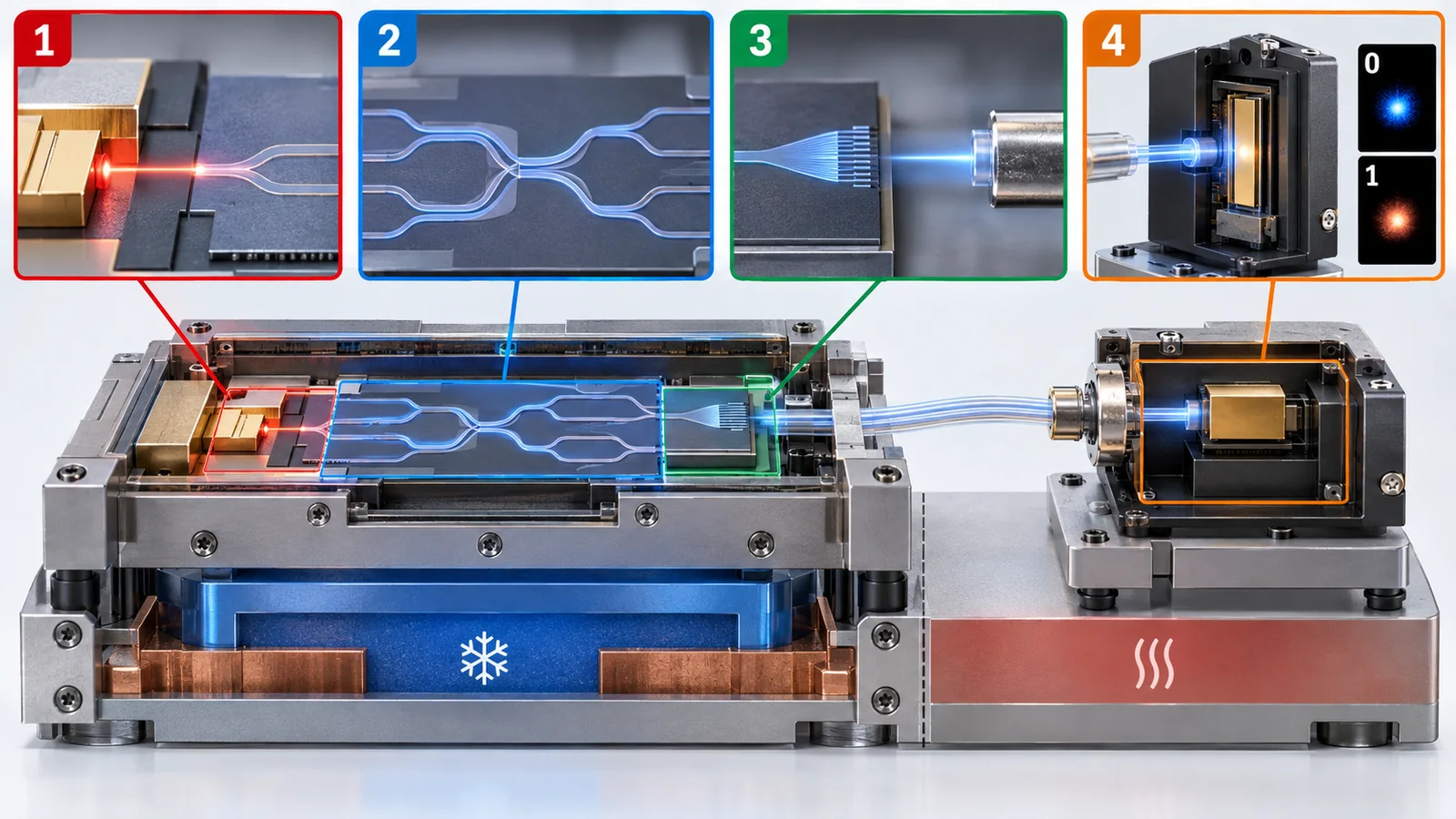
View original SVG, values and sources
Original SVG reference: Concept diagram (vector drawing). Concept diagram of a photonic quantum chip and its materials and temperature issues. The values are from Alexander et al. [Ref. 6] (values reported by a company team).
Temperature: the circuit at room temperature, the detectors cooled
Aghaee Rad et al. state that photonic quantum computers have the advantage that "most components run at room temperature"[Ref. 2]Sourced. But in practice detectors that count photons one at a time are often cooled. In PsiQuantum's example, superconducting nanowire single-photon detectors (SNSPDs) run at about 2 K, with a roughly 5 nm niobium-nitride (NbN) film and hairpin-shaped wires about 90 nm wide introduced into the silicon-photonics stack[Ref. 6]Sourced. In the continuous-variable work of Konno et al., the light states are generated at room temperature and atmospheric pressure[Ref. 10]Sourced. For detectors that count photon numbers, the Furusawa project of the JST Moonshot program lists the development of a superconducting photon-number discriminator[Ref. 36]Sourced. So "photonic means room temperature" should accurately be read as most of the circuit is at room temperature, while detectors often need cooling (commentary). Detector materials and cooling are covered in our explainer on photodetectors.
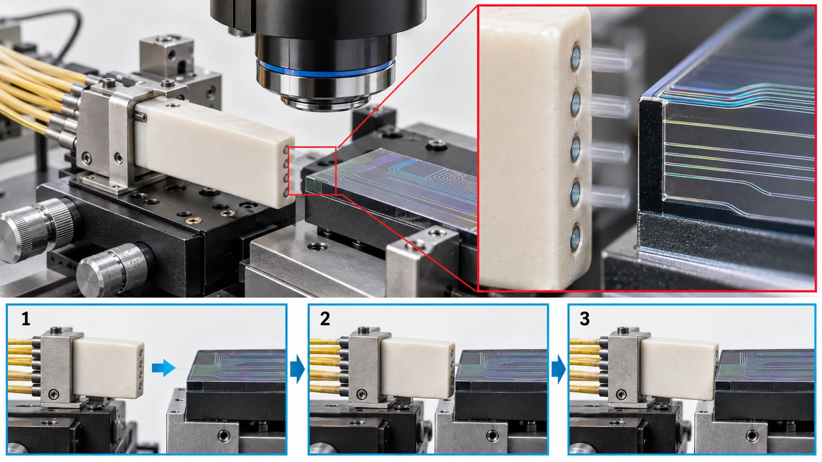
As the calculation in Chapter 6 shows, a practical starting point for a photonic quantum computer is to bring the loss per component to the order of 0.1% (Our calculation). Scattering from sidewall roughness of waveguides, optical absorption of materials and coupling loss at fiber-to-chip connections translate directly into photon loss. That is why PsiQuantum's paper lists silicon nitride waveguides, with lower loss than silicon waveguides, among its next-generation parts[Ref. 6]Sourced. A Xanadu team made GKP states with an ultra-low-loss chip built on a 300 mm wafer multilayer silicon nitride platform[Ref. 11]Sourced. These materials and their manufacturing are covered in our explainers on silicon nitride waveguides, silicon photonics and thin-film lithium niobate. For a materials engineer, a photonic quantum computer is a field that uses telecom optical-materials technology against a loss standard orders of magnitude stricter (commentary).
The HOM visibility gauges how identical photons are, so manufacturing variation of the photon source translates directly into gate quality. The PsiQuantum team lists "fabrication-tolerant photon sources" among its next-generation parts[Ref. 6]Sourced. The source's laser (pump light) is orders of magnitude stronger than the photons, so on-chip filters remove it by 99.1 ± 1.2 dB and the detectors are further encased in metal to protect them from scattered light (about 115 dB of pump suppression was observed)[Ref. 6]Sourced. Inference: this suggests that the materials challenge of photonics extends beyond loss to materials technology for shielding, filters and multilayer wiring — how to block strong light next to a detector.
9. Where things stand (checked 16 October 2026), plans, and claims of quantum advantage
(1) Peer-reviewed papers by company research teams
PsiQuantum (Alexander et al., Nature 2025): as in Chapter 8, a manufacturable platform and fidelities that do not account for loss[Ref. 6]Sourced. Xanadu: Aghaee Rad et al. (Nature 2025) built Aurora, a "(sub-performant) scale model" of a quantum computer using 35 photonic chips, 84 squeezers and 36 photon-number-resolving detectors to furnish 12 physical-qubit modes at each clock cycle, and showed a cluster state entangled across 86.4 billion modes and real-time decoding of a distance-2 repetition code[Ref. 2]Sourced. Larsen et al. (Nature 2025) generated GKP states on a silicon nitride chip[Ref. 11]Sourced. Quandela: Maring et al. (Nature Photonics 2024) reported, for a cloud-accessible prototype with a quantum-dot single-photon source and a reconfigurable optical chip, fidelities of 99.6 ± 0.1%, 93.8 ± 0.6% and 86 ± 1.2% for one-, two- and three-qubit gates[Ref. 1]Sourced. All are papers by company teams, and we have not confirmed reproduction by other laboratories. The paper itself calls Aurora "sub-performant."
(2) Japan: the Furusawa laboratory at the University of Tokyo and RIKEN, and the national project
RIKEN's Optical Quantum Computing Research Team (Akira Furusawa) states its final goal as "fault-tolerant large-scale universal optical quantum computers" and says it makes cluster states of optical modes larger and more precise by time-domain multiplexing[Ref. 9]Sourced. The page of the Furusawa project in the JST Moonshot R&D program aims at a large-scale optical quantum computer that operates at room temperature by 2050 and lists, as a milestone by 2030, research and development of a fault-tolerant large-scale universal machine that partly uses electrical signal processing (plans and goals)[Ref. 36]Not yet confirmed. As of the check date we could not confirm an official report that these goals have been achieved. We do not use news about companies' (startups') plans or funding, because they are not primary sources.
(3) Claims of quantum advantage and the rebuttals (who, on what, against what)
| Claim / study | What was done | Against what, and what was claimed | Cautions in reading |
|---|---|---|---|
| Jiuzhang (Zhong et al., Science 2020) | Gaussian boson sampling. 50 squeezed-light inputs fed into a 100-mode interferometer, sampled by 100 high-efficiency detectors; up to 76 photon detections observed | Claimed a sampling rate 10¹⁴ times faster than state-of-the-art simulation and supercomputers[Ref. 37]Sourced | A rebuttal points to the high photon loss of this kind of experiment and says it can be reproduced on a classical computer (next row) |
| Borealis (Madsen et al., Nature 2022, Xanadu) | Gaussian boson sampling. 216 squeezed-light modes (three-dimensional connectivity), photon-number-resolving detectors, a photonic processor programmable on all gates | Claimed that the best algorithms and supercomputers would need on average more than 9,000 years to produce one sample by exact methods, versus 36 μs for Borealis (a company team's claim)[Ref. 38]Sourced | The same paper notes that earlier photonic experiments were vulnerable to classical shortcuts (spoofing) |
| Oh et al. (Nature Physics 2024) | A classical tensor-network algorithm simulating the largest Gaussian-boson-sampling experiment so far | Complexity falls when photon loss is high; shows evidence that the classical sampler can simulate the ideal distribution better than the experiment, calling the claim of advantage into question[Ref. 12]Sourced | An "advantage" can be overturned later by progress in the best classical methods |
The arrangement is commentary; the facts in each row come from the references. These are claims of advantage on a "specific task," boson sampling, and do not mean that general-purpose quantum computing has surpassed classical computers. Our explainer on reading quantum-advantage claims covers this in detail.
Boson sampling is the task of sending photons through a linear-optical circuit and counting the output photons. Aaronson and Arkhipov (2010) gave evidence that this task cannot be simulated efficiently on a classical computer, but they also state that this model is not believed to be universal for quantum computation[Ref. 39]Sourced. So an "advantage" in boson sampling is not evidence that useful computation can be done; it means that a task that (perhaps) only a quantum device can do has been run in an experiment (commentary).
10. Limits, what we could not confirm, and a summary
(1) Full texts of standards
We did not read the full text of ISO/IEC 4879:2024, which is paid. For IEEE P7130 and P7131 we could not retrieve the IEEE pages and confirmed only the existence of the projects through StandICT.eu. We could not confirm any standard specific to photonic quantum computers.
(2) Company papers
The PsiQuantum, Xanadu and Quandela papers are by company teams, and we have not confirmed reproductions by other laboratories. The numbers are treated as values reported by company teams.
(3) Loss estimates
The loss calculation in Chapter 6 is an example for feel, not an estimate of a real machine's loss or the number of parts needed. We could not confirm a real machine's loss budget.
(4) Content not covered
We do not cover the detailed kinds of photon sources (quantum dots, spontaneous parametric down-conversion, etc.), quantum memories, quantum repeaters, or the plans of Japanese companies (startups).
(5) Progress on plans
Whether the JST Moonshot goals and companies' roadmaps have been achieved is stated only as far as official reports of achievement could be confirmed.
- A photonic quantum computer takes a single photon as a qubit. For example, which of two waveguides it is in (dual-rail) sets 0 and 1Sourced
- Photons pass through each other, so two-qubit gates are built with interference and measurement. Fusion-based quantum computation is a leading approachSourced
- Optical loss is the biggest wall. Even 0.1% per component becomes about 18% after 200 components (our calculation)Our calculation
- Strengths: robust to the environment, most of the circuit at room temperature, and linkable by optical fiber. But detectors are often cooledSourced
- "Quantum advantage" is a claim about a specific task, and rebuttals exist. It does not mean general-purpose quantum computing has surpassed classical computersSourced
11. How to read evaluations and standards
A photonic quantum computer's performance is read through photon quality (HOM visibility), gate and fusion fidelity (with or without loss), how much loss can be tolerated, and claims of quantum advantage and their rebuttals. The main caution in photonics is that a fidelity "not accounting for loss" and the quality of the whole machine including loss are different things. For standards, vocabulary has come first, while standards for how to measure performance are still at the project stage (checked 16 October 2026).
| What is evaluated | Representative benchmarks and evaluation methods (name, source) | Standards and guidance (NIST, ISO/IEC, IEEE, ETSI, ITU-T, IETF, etc.) | Cautions in reading |
|---|---|---|---|
| Photon quality (sameness) | HOM visibility. 99.50 ± 0.25% between independent sources (PsiQuantum)[Ref. 6]Sourced | We could not confirm one | The number changes with the type of photon source and measurement conditions (independent sources or the same source) |
| Gate and fusion quality | Two-qubit fusion fidelity 99.22 ± 0.12%, chip-to-chip 99.72 ± 0.04%, SPAM 99.98 ± 0.01%: values only when detection succeeds, not accounting for loss (PsiQuantum)[Ref. 6]Sourced. One-, two- and three-qubit gates 99.6%, 93.8% and 86% (Quandela)[Ref. 1]Sourced | We could not confirm one | A fidelity "not accounting for loss" is a different thing from the quality of the whole machine including loss. Always check the conditions |
| Loss and the error-correction threshold | Tolerable loss for each scheme. Examples: 10.4% per fusion (Bartolucci et al.'s ballistic scheme, under that model's conditions), the analysis of optical loss (Aghaee Rad et al.)[Ref. 5, 2]Sourced | We could not confirm one | The tolerance depends on the scheme and error-model conditions. We could not confirm a real machine's loss budget |
| Claims of quantum advantage | Boson sampling: Zhong et al. (2020), Madsen et al. (2022). Classical-side rebuttal: Oh et al. (2024)[Ref. 37, 38, 12]Sourced | We could not confirm one | Check who claims what on which task against what. If there is a re-evaluation by the best classical methods, read both side by side |
| Plans versus achievements | Goals of the JST Moonshot program (2030, 2050). We could not confirm companies' roadmaps[Ref. 36]Not yet confirmed | We could not confirm one | A goal is not an achieved fact. Check whether the figure is physical or logical |
| Is the physical system a good raw material for a quantum computer? | DiVincenzo's seven items (five requirements plus two on communication): (1) many well-characterized qubits, (2) initialization, (3) coherence time much longer than a gate, (4) a universal set of gates, (5) qubit-specific measurement, (6)(7) two items on communication[Ref. 41]Sourced | We could not confirm one (this is a paper's framework, not a standard) | It is a checklist, not a score. Each of the four approaches meets the items in different ways and has different weak points |
| Gate accuracy (one- and two-qubit) | Randomized benchmarking (RB): run random gate sequences and infer the average error from how success decays (Knill et al., 2008; Magesan et al., 2011)[Ref. 42, 43]Sourced | IEEE P7131 (quantum computing performance metrics and benchmarking) is at the project stage[Ref. 44]Not yet confirmed | Read "99.9% fidelity" together with which operation was measured and how. RB numbers depend on how the test is done |
| Quality of the whole machine | Quantum volume (Cross et al., 2019), EPLG (McKay et al., 2023), CLOPS (Wack et al., 2021), a method to measure capabilities (Proctor et al., 2022)[Ref. 45, 29, 46, 47]Sourced | We could not confirm one (IEEE P7131 is at the project stage)[Ref. 44]Not yet confirmed | Each metric measures something different. Do not decide a machine's merit from one number (a survey of benchmarks: Acuaviva et al., 2026[Ref. 48]) |
| Terminology and definitions | — (a vocabulary standard, not an evaluation method) | ISO/IEC 4879:2024 "Information technology — Quantum computing — Vocabulary" (first edition, May 2024, published)[Ref. 40]Sourced. IEEE P7130 (quantum technology definitions) is at the project stage[Ref. 49]Not yet confirmed | The standards' full texts are paid, so we did not read them. We do not state their requirements or definitions |
The arrangement of the table is Our calculation (organization). Because the standards' full texts are paid, we give only titles and status (checked 16 October 2026).
Cautions in reading (for materials engineers)
- "How many qubits" alone does not tell performance. Aurora's "12 physical-qubit modes" and PsiQuantum's "dual-rail qubits" are counted differently[Ref. 2, 6]
- A fidelity "not accounting for loss" is not the quality of the whole machine. In photonics, loss is the biggest challenge, so always check the figure that includes loss[Ref. 6, 2]
- A company's announcement and third-party verification are different. Read claims of quantum advantage together with classical-side rebuttals.[Ref. 38, 12]
- Check whether a standard is a recommendation or a requirement, and whether it is legally binding. ISO/IEC 4879 is a vocabulary standard and does not guarantee performance[Ref. 40]. Plans are Not yet confirmed
12. Glossary
- Qubit
- The unit of information in a quantum computer. It can point in a direction between 0 and 1. In the series' shared picture, an "arrow."
- Photon
- A particle of light. In a photonic quantum computer a single photon is a qubit.
- Waveguide
- A path for light inside a chip that confines and guides it.
- Dual-rail
- A way to represent 0 and 1 by which of two waveguides holds the photon.
- Beam splitter (BS)
- A half-silvered mirror that divides light in two. It puts a photon in a superposition.
- Phase shifter
- A part that shifts the phase of light. Used to turn the arrow.
- Interference
- The adding of light waves (reinforcing and cancelling).
- HOM interference
- The phenomenon in which two indistinguishable photons leave a beam splitter on the same side. A gauge of photons' sameness.
- Linear optics
- Optics built from parts such as beam splitters and phase shifters in which light does not interact with light.
- KLM scheme
- The scheme showing that scalable quantum computing is possible with single photons, linear optics and measurement alone (2001).
- Measurement-based (one-way) quantum computing
- A scheme that prepares a large entangled state in advance and computes just by measuring one qubit after another.
- Fusion
- An operation that takes one photon from each of two resource states, interferes and measures them, and links the two.
- Resource state
- A small entangled state that serves as material for computation.
- Photon loss
- Photons being lost through scattering, absorption and so on. The biggest challenge of photonic quantum computers.
- Photon-number-resolving detector (PNR)
- A detector that can count the number of photons.
- Superconducting nanowire single-photon detector (SNSPD)
- A high-efficiency single-photon detector that operates at cryogenic temperature.
- Squeezed light
- Light whose wave fluctuation is reduced in one direction. Used in the continuous-variable approach.
- Homodyne detection
- Detection that measures the amplitude of a light wave. Used in the continuous-variable approach.
- GKP qubit
- A qubit placed in a single light wave in an error-robust form.
- Time-domain multiplexing
- A way of lining up light pulses in time so one optical system is used repeatedly.
- Gaussian boson sampling
- The task of sending squeezed light through an interferometer and counting the output photons. Not general-purpose computation.
- Claim of quantum advantage
- A claim that a specific task is faster than on a classical computer. Classical-side rebuttals may exist.
13. References (primary sources)
- Maring N. et al. (Quandela) "A versatile single-photon-based quantum computing platform", Nat. Photon. 18, 603–609 (2024), DOI 10.1038/s41566-024-01403-4 — doi.org/10.1038/s41566-024-01403-4
- Aghaee Rad J. et al. (Xanadu) "Scaling and networking a modular photonic quantum computer", Nature 638, 912–919 (2025), DOI 10.1038/s41586-024-08406-9 — doi.org/10.1038/s41586-024-08406-9
- Kok P. et al. "Linear optical quantum computing with photonic qubits", Rev. Mod. Phys. 79, 135–174 (2007), DOI 10.1103/RevModPhys.79.135 — doi.org/10.1103/RevModPhys.79.135
- Knill E., Laflamme R., Milburn G. J. "A scheme for efficient quantum computation with linear optics", Nature 409, 46–52 (2001), DOI 10.1038/35051009 — doi.org/10.1038/35051009
- Bartolucci S. et al. (PsiQuantum) "Fusion-based quantum computation", Nat. Commun. 14, 912 (2023), DOI 10.1038/s41467-023-36493-1 — doi.org/10.1038/s41467-023-36493-1
- Alexander K. et al. (PsiQuantum) "A manufacturable platform for photonic quantum computing", Nature 641, 876–883 (2025), DOI 10.1038/s41586-025-08820-7 (we also read the arXiv:2404.17570 version) — doi.org/10.1038/s41586-025-08820-7
- Raussendorf R., Briegel H. J. "A one-way quantum computer", Phys. Rev. Lett. 86, 5188–5191 (2001), DOI 10.1103/PhysRevLett.86.5188 — doi.org/10.1103/PhysRevLett.86.5188
- Asavanant W. et al. "Generation of time-domain-multiplexed two-dimensional cluster state", Science 366, 373–376 (2019), DOI 10.1126/science.aay2645 — doi.org/10.1126/science.aay2645
- RIKEN Center for Quantum Computing "Optical Quantum Computing Research Team" (official page; checked 16 October 2026) — www.riken.jp/en/research/labs/rqc/opt_qtm_comput_res/
- Konno S. et al. "Logical states for fault-tolerant quantum computation with propagating light", Science 383, 289–293 (2024), DOI 10.1126/science.adk7560 — doi.org/10.1126/science.adk7560
- Larsen M. V. et al. (Xanadu) "Integrated photonic source of Gottesman–Kitaev–Preskill qubits", Nature 642, 587–591 (2025), DOI 10.1038/s41586-025-09044-5 — doi.org/10.1038/s41586-025-09044-5
- Oh C. et al. "Classical algorithm for simulating experimental Gaussian boson sampling", Nat. Phys. 20, 1461–1468 (2024), DOI 10.1038/s41567-024-02535-8 — doi.org/10.1038/s41567-024-02535-8
- Krantz P. et al. "A quantum engineer's guide to superconducting qubits", Appl. Phys. Rev. 6, 021318 (2019), DOI 10.1063/1.5089550 — doi.org/10.1063/1.5089550
- Bruzewicz C. D. et al. "Trapped-ion quantum computing: Progress and challenges", Appl. Phys. Rev. 6, 021314 (2019), DOI 10.1063/1.5088164 — doi.org/10.1063/1.5088164
- Ransford A. et al. (Quantinuum) "A 98-qubit trapped-ion quantum computer with all-to-all connectivity", Nature 655, 81–86 (2026), DOI 10.1038/s41586-026-10676-4 (we read the preprint arXiv:2511.05465 "Helios: A 98-qubit trapped-ion quantum computer") — doi.org/10.1038/s41586-026-10676-4
- Evered S. J. et al. "High-fidelity parallel entangling gates on a neutral-atom quantum computer", Nature 622, 268–272 (2023), DOI 10.1038/s41586-023-06481-y (we also read the arXiv:2304.05420 version) — doi.org/10.1038/s41586-023-06481-y
- Ma S. et al. "High-fidelity gates and mid-circuit erasure conversion in an atomic qubit", Nature 622, 279–284 (2023), DOI 10.1038/s41586-023-06438-1 — doi.org/10.1038/s41586-023-06438-1
- Radnaev A. G. et al. (Infleqtion) "A universal neutral-atom quantum computer with individual optical addressing and non-destructive readout", PRX Quantum 6, 030334 (2025), DOI 10.1103/66s8-jj18 — doi.org/10.1103/66s8-jj18
- IBM "IBM Quantum — Technology" (official page; checked 16 October 2026) — www.ibm.com/quantum/technology
- Sørensen A., Mølmer K. "Quantum computation with ions in thermal motion", Phys. Rev. Lett. 82, 1971–1974 (1999), DOI 10.1103/PhysRevLett.82.1971 — doi.org/10.1103/PhysRevLett.82.1971
- Löschnauer C. M. et al. (Oxford Ionics) "Scalable, high-fidelity all-electronic control of trapped-ion qubits", PRX Quantum 6, 040313 (2025), DOI 10.1103/h4wk-v31j — doi.org/10.1103/h4wk-v31j
- Saffman M., Walker T. G., Mølmer K. "Quantum information with Rydberg atoms", Rev. Mod. Phys. 82, 2313–2363 (2010), DOI 10.1103/RevModPhys.82.2313 — doi.org/10.1103/RevModPhys.82.2313
- Blais A. et al. "Circuit quantum electrodynamics", Rev. Mod. Phys. 93, 025005 (2021), DOI 10.1103/RevModPhys.93.025005 — doi.org/10.1103/RevModPhys.93.025005
- Wallraff A. et al. "Strong coupling of a single photon to a superconducting qubit using circuit quantum electrodynamics", Nature 431, 162–167 (2004), DOI 10.1038/nature02851 — doi.org/10.1038/nature02851
- Manetsch H. J. et al. "A tweezer array with 6,100 highly coherent atomic qubits", Nature 647, 60–67 (2025), DOI 10.1038/s41586-025-09641-4 (we read the abstract of the arXiv:2403.12021 version) — doi.org/10.1038/s41586-025-09641-4
- Ballance C. J. et al. "High-fidelity quantum logic gates using trapped-ion hyperfine qubits", Phys. Rev. Lett. 117, 060504 (2016), DOI 10.1103/PhysRevLett.117.060504 — doi.org/10.1103/PhysRevLett.117.060504
- Mehta K. K. et al. "Integrated optical multi-ion quantum logic", Nature 586, 533–537 (2020), DOI 10.1038/s41586-020-2823-6 — doi.org/10.1038/s41586-020-2823-6
- Bluvstein D. et al. "A fault-tolerant neutral-atom architecture for universal quantum computation", Nature 649, 39–46 (2025), DOI 10.1038/s41586-025-09848-5 (we read the abstract of the arXiv:2506.20661 version) — doi.org/10.1038/s41586-025-09848-5
- McKay D. C. et al. "Benchmarking quantum processor performance at scale", arXiv:2311.05933 (preprint, November 2023) — arxiv.org/abs/2311.05933
- Bluvstein D. et al. "A quantum processor based on coherent transport of entangled atom arrays", Nature 604, 451–456 (2022), DOI 10.1038/s41586-022-04592-6 — doi.org/10.1038/s41586-022-04592-6
- Google Quantum AI, Acharya R. et al. "Quantum error correction below the surface code threshold", Nature 638, 920–926 (2025), DOI 10.1038/s41586-024-08449-y (we also read the arXiv:2408.13687 version) — doi.org/10.1038/s41586-024-08449-y
- Bland M. P. et al. "Millisecond lifetimes and coherence times in 2D transmon qubits", Nature 647, 343–348 (2025), DOI 10.1038/s41586-025-09687-4 (we also read the arXiv:2503.14798 version) — doi.org/10.1038/s41586-025-09687-4
- Krinner S. et al. "Engineering cryogenic setups for 100-qubit scale superconducting circuit systems", EPJ Quantum Technol. 6, 2 (2019), DOI 10.1140/epjqt/s40507-019-0072-0 — doi.org/10.1140/epjqt/s40507-019-0072-0
- Zhang E. J. et al. "High-fidelity superconducting quantum processors via laser-annealing of transmon qubits", arXiv:2012.08475 (published as Sci. Adv. 8, eabi6690 (2022); we read the abstract of the arXiv version) — arxiv.org/abs/2012.08475
- Chiu N.-C. et al. "Continuous operation of a coherent 3,000-qubit system", Nature 646, 1075–1080 (2025), DOI 10.1038/s41586-025-09596-6 — doi.org/10.1038/s41586-025-09596-6
- JST Moonshot R&D Program "Goal 6: FURUSAWA Akira Project — Development of Large-scale Fault-tolerant Universal Optical Quantum Computers" (official page, last updated 15 September 2026; checked 16 October 2026) — www.jst.go.jp/moonshot/en/program/goal6/64_furusawa.html
- Zhong H.-S. et al. "Quantum computational advantage using photons", Science 370, 1460–1463 (2020), DOI 10.1126/science.abe8770 — doi.org/10.1126/science.abe8770
- Madsen L. S. et al. (Xanadu) "Quantum computational advantage with a programmable photonic processor", Nature 606, 75–81 (2022), DOI 10.1038/s41586-022-04725-x — doi.org/10.1038/s41586-022-04725-x
- Aaronson S., Arkhipov A. "The computational complexity of linear optics", arXiv:1011.3245 (Theory of Computing 9, 143 (2013)) — arxiv.org/abs/1011.3245
- ISO/IEC "ISO/IEC 4879:2024 Information technology — Quantum computing — Vocabulary" (ISO page; first edition, May 2024, published) — www.iso.org/standard/80432.html
- DiVincenzo D. P. "The physical implementation of quantum computation", Fortschr. Phys. 48, 771–783 (2000), arXiv:quant-ph/0002077 — arxiv.org/abs/quant-ph/0002077
- Knill E. et al. "Randomized benchmarking of quantum gates", Phys. Rev. A 77, 012307 (2008), DOI 10.1103/PhysRevA.77.012307 — doi.org/10.1103/PhysRevA.77.012307
- Magesan E., Gambetta J. M., Emerson J. "Scalable and robust randomized benchmarking of quantum processes", Phys. Rev. Lett. 106, 180504 (2011), DOI 10.1103/PhysRevLett.106.180504 — doi.org/10.1103/PhysRevLett.106.180504
- StandICT.eu "P7131 - Standard for Quantum Computing Performance Metrics & Performance Benchmarking" (an IEEE project, as listed in the StandICT.eu standards repository; the IEEE page itself could not be retrieved) — standict.eu/standards-repository/p7131-standard-quantum-computing-performance-metrics-performance-benchmarking
- Cross A. W. et al. "Validating quantum computers using randomized model circuits", Phys. Rev. A 100, 032328 (2019), DOI 10.1103/PhysRevA.100.032328 — doi.org/10.1103/PhysRevA.100.032328
- Wack A. et al. "Quality, speed, and scale: three key attributes to measure the performance of near-term quantum computers", arXiv:2110.14108 (preprint, October 2021) — arxiv.org/abs/2110.14108
- Proctor T. et al. "Measuring the capabilities of quantum computers", Nat. Phys. 18, 75–79 (2022), DOI 10.1038/s41567-021-01409-7 — doi.org/10.1038/s41567-021-01409-7
- Acuaviva A. et al. "Benchmarking quantum computers: towards a standard performance evaluation approach", Quantum Sci. Technol. 11, 025004 (2026), DOI 10.1088/2058-9565/ae4269 — doi.org/10.1088/2058-9565/ae4269
- StandICT.eu "P7130 - Standard for Quantum Technologies Definitions" (an IEEE project, as listed in the StandICT.eu standards repository; the IEEE page itself could not be retrieved) — standict.eu/standards-repository/p7130-standard-quantum-technologies-definitions
14. Claim-to-source audit
| Claim in the text | Basis | Type |
|---|---|---|
| PsiQuantum (Alexander et al.): dual-rail SPAM 99.98 ± 0.01%, HOM visibility 99.50 ± 0.25%, two-qubit fusion 99.22 ± 0.12%, chip-to-chip 99.72 ± 0.04% (conditional on detection, not accounting for loss), 300 mm silicon photonics, SNSPDs (NbN about 5 nm, about 90 nm wide, about 2 K), pump suppression 99.1 ± 1.2 dB and about 115 dB, next-generation parts (SiN, BTO, PNR detectors, fiber coupling, fabrication-tolerant photon sources) | Alexander et al. (text of the arXiv version, abstract of the Nature paper) Reference 6 https://doi.org/10.1038/s41586-025-08820-7 | Sourced |
| Aghaee Rad et al. (Xanadu): 35 chips, 84 squeezers, 36 PNR detectors, 12 physical-qubit modes per clock, a cluster state over 86.4 billion modes, a distance-2 repetition code, a "sub-performant scale model," most components at room temperature, optical loss as the dominant and most challenging hurdle | Abstract on the Nature paper page Reference 2 https://doi.org/10.1038/s41586-024-08406-9 | Sourced |
| Larsen et al. (Xanadu): GKP states on a silicon nitride chip (300 mm wafer, multilayer), negative Wigner-function regions in a 3×3 grid, possibly reaching the fault-tolerant regime after further loss reduction | Abstract on the Nature paper page Reference 11 https://doi.org/10.1038/s41586-025-09044-5 | Sourced |
| Maring et al. (Quandela): quantum-dot photon source, a reconfigurable optical chip, one-, two- and three-qubit gates at 99.6 ± 0.1%, 93.8 ± 0.6% and 86 ± 1.2%, and the advantages of photonics (low decoherence, modest cryogenic requirements) | Abstract on the Nature Photonics paper page Reference 1 https://doi.org/10.1038/s41566-024-01403-4 | Sourced |
| The KLM scheme (2001), measurement-based quantum computing (2001), fusion-based quantum computation (a ballistic scheme tolerating 10.4% loss per fusion), the review of photonic quantum computing, and Bourassa et al. (a design for a room-temperature photonic computer) | Bibliographic records and abstracts Reference 4 https://doi.org/10.1038/35051009 Reference 7 https://doi.org/10.1103/PhysRevLett.86.5188 Reference 5 https://doi.org/10.1038/s41467-023-36493-1 Reference 3 https://doi.org/10.1103/RevModPhys.79.135 | Sourced |
| Konno et al.: a GKP state in propagating light at a telecom wavelength, homodyne measurement without loss correction, room temperature and atmospheric pressure. Asavanant et al.: a time-domain-multiplexed two-dimensional cluster state. RIKEN's optical team: final goal and time-domain multiplexing. JST Moonshot: a large-scale machine operating at room temperature by 2050, the 2030 milestone, a superconducting photon-number discriminator | Abstracts of each paper, and the official pages of RIKEN and JST (checked 16 October 2026) Reference 10 https://doi.org/10.1126/science.adk7560 Reference 8 https://doi.org/10.1126/science.aay2645 Reference 9 https://www.riken.jp/en/research/labs/rqc/opt_qtm_comput_res/ Reference 36 https://www.jst.go.jp/moonshot/en/program/goal6/64_furusawa.html | Sourced |
| Zhong et al. (Jiuzhang): 50 squeezed-light inputs, 100 modes, 100 detectors, 76 photons, 10¹⁴ times. Madsen et al. (Borealis): 216 modes, over 9,000 years versus 36 μs, earlier photonic experiments vulnerable to spoofing. Oh et al.: classical tensor-network simulation, complexity falls with high loss, calling the advantage claim into question. Aaronson and Arkhipov: boson sampling is not believed to be universal | Abstracts of each paper Reference 37 https://doi.org/10.1126/science.abe8770 Reference 38 https://doi.org/10.1038/s41586-022-04725-x Reference 12 https://doi.org/10.1038/s41567-024-02535-8 Reference 39 https://arxiv.org/abs/1011.3245 | Sourced |
| DiVincenzo's framework of five requirements (plus two on communication) | Abstract and text of DiVincenzo (2000) Reference 41 https://arxiv.org/abs/quant-ph/0002077 | Sourced |
| Existence and titles of the original randomized-benchmarking papers (Knill et al.; Magesan et al.) | Bibliographic records (checked via Crossref / the publisher's page) Reference 42 https://doi.org/10.1103/PhysRevA.77.012307 Reference 43 https://doi.org/10.1103/PhysRevLett.106.180504 | Sourced |
| Titles and abstracts of the papers on quantum volume, EPLG, CLOPS, capability measurement and the benchmarking survey | Abstracts of each paper Reference 45 https://doi.org/10.1103/PhysRevA.100.032328 Reference 29 https://arxiv.org/abs/2311.05933 Reference 46 https://arxiv.org/abs/2110.14108 Reference 47 https://doi.org/10.1038/s41567-021-01409-7 Reference 48 https://doi.org/10.1088/2058-9565/ae4269 | Sourced |
| Number, title and publication date of ISO/IEC 4879:2024 (first edition, May 2024, published) | ISO page Reference 40 https://www.iso.org/standard/80432.html | Sourced |
| IEEE P7130 and P7131 exist as IEEE projects (we treat their status as project stage and do not call them settled standards) | Listing in the StandICT.eu standards repository (the IEEE page itself could not be retrieved) Reference 49 https://standict.eu/standards-repository/p7130-standard-quantum-technologies-definitions Reference 44 https://standict.eu/standards-repository/p7131-standard-quantum-computing-performance-metrics-performance-benchmarking | Not yet confirmed |
| Facts on other approaches (the four-approach table): the review by Krantz et al., Willow and IBM, ions such as Helios and Ballance et al., neutral atoms such as Evered et al., and others | Abstracts, texts and official pages Reference 13 https://doi.org/10.1063/1.5089550 Reference 31 https://doi.org/10.1038/s41586-024-08449-y Reference 32 https://doi.org/10.1038/s41586-025-09687-4 Reference 33 https://doi.org/10.1140/epjqt/s40507-019-0072-0 Reference 34 https://arxiv.org/abs/2012.08475 Reference 19 https://www.ibm.com/quantum/technology Reference 14 https://doi.org/10.1063/1.5088164 Reference 15 https://doi.org/10.1038/s41586-026-10676-4 Reference 20 https://doi.org/10.1103/PhysRevLett.82.1971 Reference 21 https://doi.org/10.1103/h4wk-v31j Reference 26 https://doi.org/10.1103/PhysRevLett.117.060504 Reference 27 https://doi.org/10.1038/s41586-020-2823-6 Reference 16 https://doi.org/10.1038/s41586-023-06481-y Reference 17 https://doi.org/10.1038/s41586-023-06438-1 Reference 18 https://doi.org/10.1103/66s8-jj18 Reference 22 https://doi.org/10.1103/RevModPhys.82.2313 Reference 25 https://doi.org/10.1038/s41586-025-09641-4 Reference 30 https://doi.org/10.1038/s41586-022-04592-6 Reference 28 https://doi.org/10.1038/s41586-025-09848-5 Reference 35 https://doi.org/10.1038/s41586-025-09596-6 Reference 23 https://doi.org/10.1103/RevModPhys.93.025005 Reference 24 https://doi.org/10.1038/nature02851 Reference 29 https://arxiv.org/abs/2311.05933 | Sourced |
| Total loss by 1−(1−ℓ)ⁿ (0.1%: 100 components give 9.5% and 200 give 18.1%; the numbers of components reaching 10.4% are about 110, 22 and 11) | Our calculation (Python; inputs are conceptual examples; 10.4% is Bartolucci et al.'s value) | Our calculation |
| Explanations, analogies and the materials engineer's views such as "photons pass through each other," the explanation of HOM interference, "a photon keeps travelling," "loss sways the value of gates," materials and shielding issues, and "boson sampling is not general-purpose," plus the "In three lines" and "common misconception" boxes | This article's organization and commentary based on published content (our own explanation). Not views expressed by the institutions concerned | Commentary |
| Figures 1 and 11 being ImageGen-generated conceptual illustrations; the other figures being drawings made to explain, not observations of real data | A note in this article (our own) | Commentary |
| Not confirmed: the full texts of ISO/IEC and IEEE standards, the IEEE official pages, any standard specific to photonic quantum computers, reproductions of company teams' results by other laboratories, loss budgets, companies' roadmaps, and achievement of the Moonshot goals | Could not be confirmed in the primary sources accessible within this study, so not stated (our own) | Commentary |
Last updated: 16 October 2026. Sources are limited to primary ones (peer-reviewed papers, arXiv papers, and the official pages of ISO, RIKEN and JST). The standards' full texts are paid and were not read. The loss calculation is our own feel-for-the-size example, not the loss of any real machine. We could not confirm reproductions of company teams' results by other laboratories, the IEEE official pages, loss budgets, companies' roadmaps, or achievement of the Moonshot goals, so we do not state them. All figures are explanatory concept diagrams or drawings that include our own calculations; Figures 1 and 11 are ImageGen-generated conceptual illustrations.