TECHNOLOGY EXPLAINER
Trapped Ions
― How a single atom floated by electric forces becomes a qubit, and the materials and optics behind it
The trapped-ion approach floats atoms (ions) in vacuum with electric forces and turns them into qubits one by one. An ion is an atom made by nature, so ions of one species are all exactly alike; that is why laser light or microwaves can control them very precisely. In exchange, gates are slow, and scaling up demands clever work on electrodes, lasers and wiring. This article explains, step by step with figures and small numerical examples: (1) how an ion is floated, (2) why two states inside an atom make a qubit, (3) how it is controlled and read out, (4) strengths and weaknesses, (5) a way to scale up (the QCCD approach), and (6) the materials, optics and vacuum behind it. The later chapters summarize the state of play as of the check date (16 October 2026), keeping achievements and plans apart.
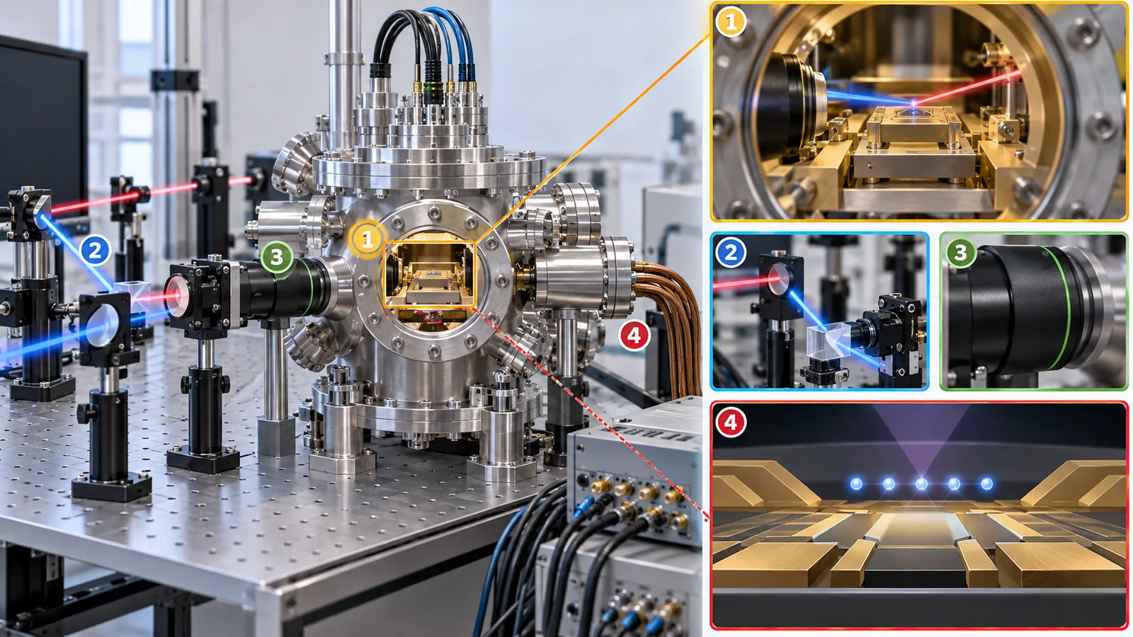
- In three lines / what to know first / where this sits in the series
- Recap: a qubit is an "arrow"
- How is an ion floated? (the Paul trap)
- The qubit is "two states inside an atom"
- Control: one-qubit and two-qubit gates
- Readout: bright or dark
- The key points on a common "card," and a side-by-side with the other three approaches
- Scaling up: the QCCD that moves ions, and wiring
- Materials, optics and vacuum
- Where things stand (checked 16 October 2026) and plans
- Limits, what we could not confirm, and a summary
- How to read evaluations and standards
- Glossary
- References (primary sources)
- Claim-to-source audit
Sourced = stated in a published source (with a link)
Our calculation = a value this article computed from stated assumptions
Not yet confirmed = plans, targets, drafts and other items that are not settled
Readings for materials research and analogies are marked as commentary. An inference is shown in bold.
A quantum-computing number means little unless it comes with what was measured and how. Here, error rates, fidelities and lifetimes come with the approach, the thing measured, whether it is an average or a best value, and the date. Company announcements are labeled as the company's claims, and plans and targets are shown as Not yet confirmed, kept apart from achieved facts. The numerical example in the readout figure is our own assumed "feel-for-the-size" example, not the performance of any real machine. We did not read the full texts of the standards (ISO/IEC, IEEE), which are paid; we give only titles and status. We do not tell lies to keep things simple. Every analogy comes with its limits.
1. In three lines / what to know first / where this sits in the series
- A trapped-ion qubit is a single atomic ion floated in vacuum by electric fields. 0 and 1 are two internal states of that atom (for example, hyperfine levels)[Ref. 1, 2]Sourced
- Ions of one species are all identical and can be controlled precisely with laser light or microwaves. High precision has been reported, such as an average two-qubit-gate infidelity of 7.9×10⁻⁴ (average over all zones of a 98-qubit machine). On the other hand, gates are slow (about 70 μs in one example)[Ref. 2, 1]Sourced
- Scaling up brings the difficulty of more electrodes, lasers and wiring. The QCCD approach that moves ions around, optics built into the chip, and control by electrical signals are advancing as answers[Ref. 3, 4, 5, 6]Sourced
Trapped ions use "identical atoms made by nature" as qubits, so precision is high. In exchange, gates are slow, and scaling up requires "moving ions around and integrating light and electrodes into the chip."
Prerequisites: none. The arrow picture is recapped in the next chapter (no quantum-mechanics formulas are used).
Place in the series: read this after "The Basics of Quantum Computing" and "Quantum Gates and Circuits." It is easiest to read side by side with the other three approaches (superconducting, neutral atoms, photonic quantum computers). How error rates and lifetimes are measured is in our explainer on coherence and fidelity; vacuum and cryogenic techniques in our explainer on cryogenics and control; materials in general in our explainer on materials and manufacturing for quantum computers; and optical components in our explainers on optical fiber, silicon nitride waveguides, silicon photonics, photodetectors and semiconductor lasers.
2. Recap: a qubit is an "arrow"
In this series, a qubit's state is drawn as an arrow from the center of a sphere to its surface. Pointing at the north pole means "0," pointing at the south pole means "1," and pointing in between is a superposition. When the arrow is tilted, a measurement always gives 0 or 1, and the chance of each is set by the tilt. After the measurement the arrow is fixed at a pole, and the old tilt does not come back.
That is wrong. A tilted arrow is not "holding both 0 and 1" but "pointing in a definite direction between 0 and 1." Measure it and you get just one of 0 or 1. A quantum computer's power comes from combining these arrow directions like waves so that the right answer reinforces itself (see our explainer on quantum algorithms).
3. How is an ion floated? (the Paul trap)
(1) Why an "ion"?
An atom is electrically neutral, so an electric field cannot grab it. So one electron is stripped away to make a positively charged "ion." Because it carries charge, electric fields can push and pull it and hold it in mid-air. Ions used for qubits include barium (Ba⁺), ytterbium (Yb⁺) and calcium (Ca⁺)[Ref. 1, 2]Sourced.
(2) Static forces alone cannot hold it, so the field is shaken
Electric forces alone cannot confine an ion in all three directions. A "hill" always appears in some direction, and the ion rolls off (Earnshaw's theorem; commentary). So the direction of the electric field is flipped tens of millions of times per second (radio frequency, RF). On average the ion is pushed back to the center and floats between the electrodes. This is the Paul trap. It is often explained by placing a ball on a saddle-shaped surface and spinning the saddle so the ball no longer falls off (analogy; limits: the ball involves gravity and the ion electric force, and only the shape "valley and hill swap with direction" is shared).In traps for quantum computing the ion–electrode distance is 30 μm to 1 mm, the RF voltage is 10–1,000 V, and the frequency is 10–100 MHz. In ultra-high vacuum an ion can be held for hours, days and in some cases months[Ref. 1]Sourced.
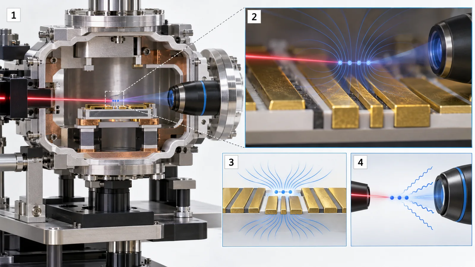
View original SVG, values and sources
Original SVG reference: Concept diagram (vector drawing). Concept diagram of how an ion is held by electric forces. The numbers come from the review by Bruzewicz et al. [Ref. 1].
(3) After floating, cool it with lasers
A floated ion is still shaking with heat. So the ion is cooled with laser light (laser cooling), using the process in which the ion absorbs and re-emits light to slow its motion. The limit of the first stage of cooling (the Doppler limit) is a few hundred μK (as explained in a technical blog by IonQ)[Ref. 7]Sourced. The important point is that even though the ion is cooled, the chip (the trap) does not need to be at a cryogenic temperature. Compared with the roughly 20 mK refrigerator of superconducting qubits, a trapped-ion trap can run at room temperature (Ballance et al. used a room-temperature trap)[Ref. 8]Sourced. Even so, a trap is sometimes cooled to about 4 K to reduce noise from the electrode surface (Chapter 9).
Trapped ions involve two kinds of cooling: cooling the machine (the chip) and cooling the ion's motion with lasers. The first can be skipped at room temperature, the second is always needed. Both are about "temperature," but an ion's "temperature" is how violently it shakes.
4. The qubit is "two states inside an atom"
An electron inside an atom can sit only on "steps" of fixed energy (energy levels). A trapped-ion qubit takes two convenient steps as 0 and 1. The commonly used pair is two steps of very close energy (hyperfine levels, separated by about a GHz), moved between with microwaves or two laser beams (a Raman transition)[Ref. 1]Sourced. A pair of a ground level and a level with a lifetime of seconds (an optical qubit) is also used[Ref. 1]Sourced.
Here is a big difference from superconducting qubits. A superconducting qubit is a circuit that people designed, and each one comes out slightly different. An ion is an atom made by nature, and all ions of the same species and isotope are identical. Every ion responds to the same microwave or laser frequency and has the same coherence time. Less tuning and high reproducibility underlie the precision of trapped ions[Ref. 1]Sourced.
Some state-holding times are very long even compared with other approaches. A 171Yb⁺ "clock-state" qubit (a state insensitive to magnetic field) holds on the order of seconds, and 600 seconds was reached with dynamical decoupling (using pulses to cancel disturbances)[Ref. 1]Sourced. In Gaebler et al.'s 9Be⁺ the memory coherence time exceeded 1 second, and Wang et al. reported a value estimated to exceed one hour for 171Yb⁺ (the paper's title says "estimated")[Ref. 9, 10]Sourced. To suppress magnetic-field fluctuations, mu-metal magnetic shielding and permanent magnets gave 300 ms (2.1 s with dynamical decoupling) in one case[Ref. 1]Sourced. These are values from different laboratories measuring different things in different ways; they are not to be set beside values of other kinds of qubits to rank them.
This is wrong. Being identical means less tuning and high reproducibility, but it does not make errors zero. Laser fluctuations, magnetic-field noise, heating of the ion and readout errors remain. Ballance et al. studied the sources of error and identified the main technical sources of two-qubit-gate infidelity[Ref. 8]Sourced. "Identical atoms" and "zero errors" are different matters.
5. Control: one-qubit and two-qubit gates
(1) One-qubit control: turning the arrow
Microwaves matched to the gap between 0 and 1 (or a frequency equal to the difference between two laser beams) turn the arrow. The pulse's length and strength set the angle. To do this to a chosen ion, the laser is focused on one ion, or the electrical signals are varied from ion to ion. Gaebler et al. lowered the one-qubit-gate error to 3.8×10⁻⁵ in 9Be⁺, and Ballance et al. showed one-qubit-gate fidelity of 99.9934(3)% in 43Ca⁺[Ref. 9, 8]Sourced. The Helios paper reports an average one-qubit-gate infidelity of 2.5×10⁻⁵[Ref. 2]Sourced.
(2) Two-qubit control: using the "shared motion" as a go-between
Ions carry the same charge and repel one another, so inside the trap's valley they sway together like beads joined by springs. A two-qubit gate connects two ions' states using this shared motion as a go-between[Ref. 1]Sourced. The idea was proposed by Cirac and Zoller in 1995[Ref. 11], and Sørensen and Mølmer showed in 1999 a form that works even with leftover thermal motion (the Mølmer–Sørensen gate)[Ref. 12]Sourced.
Examples of precision (definitions and conditions differ): Ballance et al. studied two-qubit-gate fidelity of 99.9(1)% in a room-temperature trap with 43Ca⁺ over gate times of 3.8 μs to 520 μs, showing that going faster lowers fidelity (a speed–precision trade-off)[Ref. 8]Sourced. Gaebler et al. estimated the two-qubit-gate error in 9Be⁺ as 8(4)×10⁻⁴[Ref. 9]Sourced. The paper on Quantinuum's Helios (98 qubits) reports an average two-qubit-gate infidelity of 7.9(2)×10⁻⁴ (average over all zones) and an average state-preparation-and-measurement (SPAM) infidelity of 4.8(6)×10⁻⁴ (as stated in the preprint; after peer review it was published in Nature on 17 June 2026)[Ref. 2]Sourced.
Two-qubit gates in superconducting qubits take tens to hundreds of ns, while ions typically take tens of μs (about 70 μs in the Helios example), about a thousand times slower (our calculation: 70 μs ÷ 70 ns = 1,000 times; examples from different machines). Bruzewicz et al. summarize that high-fidelity two-qubit gates have been shown as fast as 1.6 μs, while the fidelity of gates faster than 1 μs has not exceeded 76% (as of 2019)[Ref. 1]Sourced. Ions, however, hold their state for a very long time, so the ratio "holding time ÷ gate time" is large. Even if slow, the qubit is unlikely to break meanwhile (commentary).
6. Readout: bright or dark
Readout in a trapped-ion machine is easy to picture. When a readout laser is applied, only ions in one state (for example |1⟩) absorb the light and keep emitting fluorescence (re-emitted light). Ions in the other state (|0⟩) do not glow and stay dark. Counting the photons (particles of light) that come out with a camera or photodetector tells you bright (1) or dark (0)[Ref. 1]Sourced. High-fidelity state preparation and readout have been done in under 1 ms[Ref. 1]Sourced.
Very little light can be collected at once. A 2019 review summarized the overall efficiency of collecting an ion's fluorescence at roughly 2–4%. Superconducting-nanowire single-photon detectors (which work only at cryogenic temperatures) have reported efficiencies of about 0.8 for ultraviolet photons[Ref. 1]Sourced. Even so, a few photons are enough to decide, so readout can be done in under 1 ms. Helios's SPAM (preparation and measurement errors together) averages 4.8×10⁻⁴[Ref. 2]Sourced. Other approaches amplify a faint resonator signal (superconducting), take a picture (neutral atoms) or count photons (photonic), whereas ions are distinctive in that you look directly at "bright or dark."
7. The key points on a common "card," and a side-by-side with the other three approaches
Here is everything so far as a "card" that answers the series' five shared questions (what it is made of, what 0 and 1 are, how it is controlled, how it is read, strengths and weaknesses). The other three articles use the same card.
Reading the four approaches in the same format
| Item | Superconducting | Trapped ion | Neutral atom | Photonic |
|---|---|---|---|---|
| What the qubit is | A superconducting circuit (e.g., a transmon): an "artificial atom" about 1 mm across, drawn on a chip[Ref. 13] | One atomic ion floated in vacuum by radio-frequency electric fields (e.g., Ba⁺, Yb⁺)[Ref. 1, 2] | One neutral atom caught in vacuum by an optical tweezer, a tightly focused laser beam (e.g., Rb, Cs, Yb)[Ref. 14, 15, 16] | A photon (a particle of light) travelling in a waveguide, a path for light, or in an optical fiber[Ref. 17, 18] |
| How 0 and 1 are told apart | The lowest two energy steps of the circuit[Ref. 13] | Two internal states of the atom (e.g., two hyperfine levels of Ba⁺)[Ref. 2] | Two internal states of the atom (e.g., two hyperfine levels of Rb)[Ref. 14] | Which of two paths the photon takes (e.g., one of two waveguides); it can also be an early or late time slot[Ref. 17, 19] |
| How it is controlled | Microwave pulses. Two-qubit gates use a coupler or the cross-resonance effect[Ref. 13, 20] | Laser light (or microwaves or electrical signals). Two-qubit gates use the shared motion of the ions as a go-between[Ref. 1, 12, 6] | Laser light. In a two-qubit gate, atoms are lifted to a highly excited Rydberg state so that nearby atoms affect each other[Ref. 21, 14] | Interference in an optical circuit and photon detection (measurement). Photons pass through each other, so measurement creates the interaction[Ref. 19, 22] |
| How it is read out | Measure a small shift in the microwave response of a resonator (dispersive readout)[Ref. 23, 24] | Shine light and see whether it fluoresces (bright / dark)[Ref. 1] | Image the fluorescence and see which atoms are bright or dark[Ref. 25] | Photodetectors count which path the photon arrived on (one example runs superconducting nanowire detectors at about 2 K)[Ref. 17] |
| Operating environment | About 20 mK in a dilution refrigerator[Ref. 13] | Ultra-high vacuum. Traps exist at room temperature and in cooled form[Ref. 8, 5] | Lasers and optics around an ultra-high-vacuum chamber. Atoms at about 10 μK, apparatus at room temperature[Ref. 14, 25] | Most circuit parts run at room temperature. Detectors are often cooled[Ref. 18, 17] |
| Example two-qubit gate time | 43 ns (an example by Barends et al.) or about 200 ns (a cross-resonance example)[Ref. 13] | About 70 μs (an example from Helios). One study scanned 3.8 μs to 520 μs[Ref. 2, 8] | Gate pulses are on the order of hundreds of ns (one calibration value in Evered et al.: 275 ns). Rearranging and imaging take longer[Ref. 14, 26] | We could not confirm a representative value |
| Example of two-qubit quality (definitions differ) | EPLG 3.7×10⁻³ as shown on IBM's official page (measurement conditions could not be confirmed)[Ref. 20, 27] | Average infidelity 7.9×10⁻⁴ (Helios, average over all zones of a 98-qubit machine)[Ref. 2] | Fidelity 99.5% (up to 60 atoms in parallel, Evered et al.)[Ref. 14] | "Fusion" fidelity 99.22% (only when detection succeeds; loss not included)[Ref. 17] |
| Strengths | Fast. Semiconductor-style microfabrication can be used[Ref. 13] | Ions of one species are all identical. Control precision is high[Ref. 1, 2] | Many identical atoms can be lined up (6,100). The layout can be changed[Ref. 25, 28] | Easy to link with optical fiber. Optical circuits can be built in a semiconductor factory (the plan)[Ref. 17, 18] |
| Weaknesses | Qubit lifetimes are relatively short. Wiring and cooling; fabrication variation[Ref. 29, 30, 31, 32] | Gates are slow. Scaling adds electrodes, lasers and wiring[Ref. 2, 1] | Atoms get lost. Cycles are slow[Ref. 33, 26] | Photon loss is the biggest challenge. Photons barely interact with each other[Ref. 18, 19] |
The arrangement is commentary; the numbers and facts in each cell come from the references (checked 16 October 2026). The numbers are different quantities under different conditions, so please do not rank the approaches by them.
The answer is "not settled yet." Each has different strengths: speed (superconducting), precision and all-to-all connectivity (ions), large numbers and freedom of layout (neutral atoms), and compatibility with communication (photons). All of them attack the same hard problem — keeping quality while adding qubits — by different routes. The numbers in this article's table have different definitions and conditions, so please do not compare them directly.
8. Scaling up: the QCCD that moves ions, and wiring
Lining ions up in a single row to add qubits runs into a limit: the more ions in one row, the slower two-qubit gates generally become (the ions are farther apart and couple more weakly to the shared motion)[Ref. 1]Sourced. So the idea arose of moving ions a few at a time. Kielpinski et al. proposed it in 2002 as the "quantum charge-coupled device (QCCD)"[Ref. 3], and Pino et al. demonstrated it in 2021 with a cooled trap chip combining all the necessary ingredients[Ref. 4]Sourced. Only the ions to be gated are carried to a logic zone, unused ions rest in a memory zone, and junctions route ions to where they need to go.
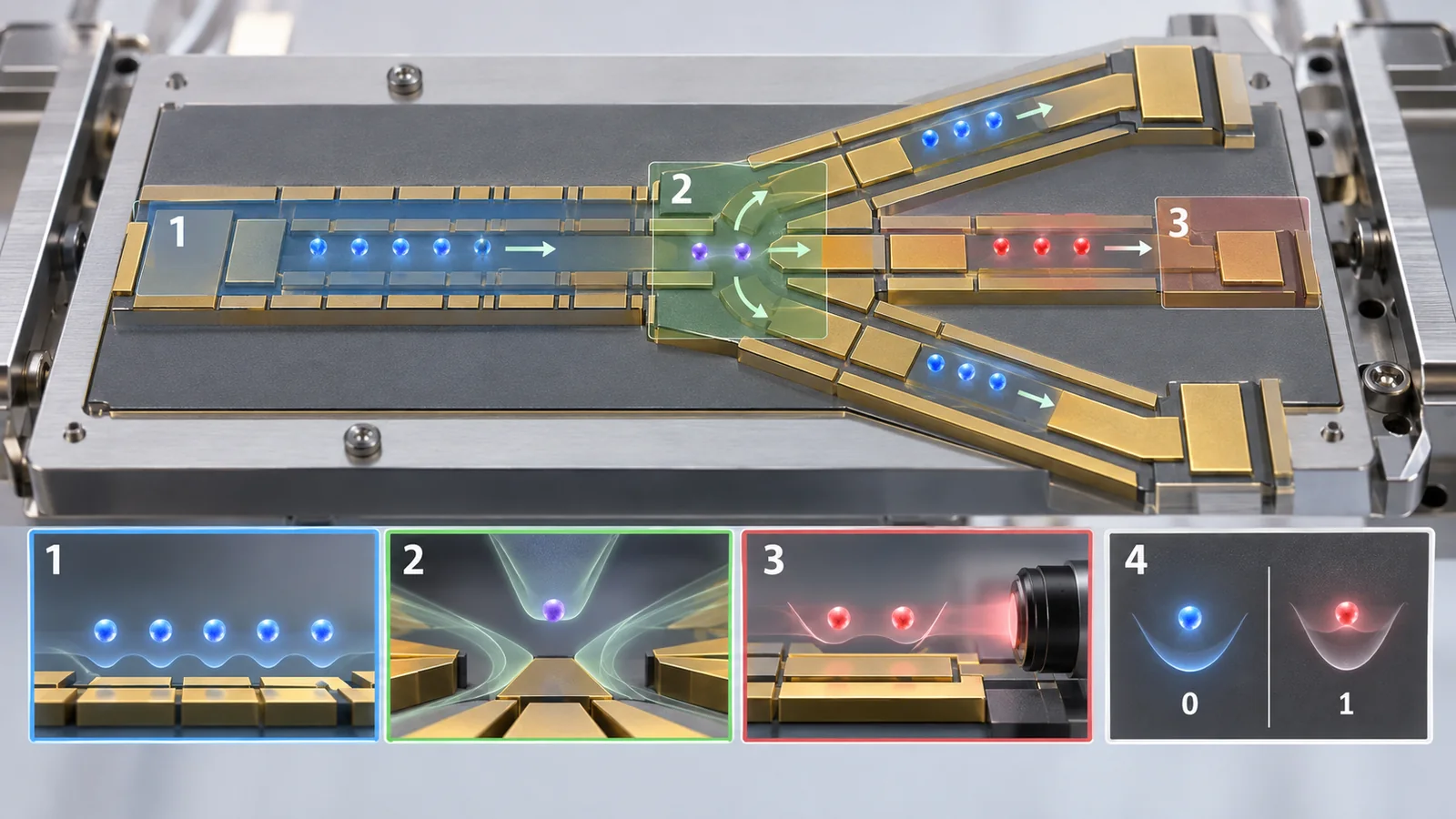
View original SVG, values and sources
Original SVG reference: Concept diagram (vector drawing). Concept diagram of the QCCD approach. Proposal and demonstration: Kielpinski et al. [Ref. 3] and Pino et al. [Ref. 4].
Helios: moving 98 ions
Quantinuum's Helios is a 98-qubit QCCD machine. It uses hyperfine levels of barium (137Ba⁺) as qubits, and a four-way "X" junction connects a rotatable ion storage ring to two logic regions. The logic region has eight zones and handles up to 16 qubits at a time. Ions heated by moving are re-cooled by cooling ytterbium (171Yb⁺) ions trapped alongside them with laser light at 369 nm, which draws off the heat (sympathetic cooling)[Ref. 2]Sourced. The two-qubit gate itself takes about 70 μs, and the paper notes an additional cooling of about 300 μs after the move[Ref. 2]Sourced.
To keep wiring from growing too much as machines scale, a design that "broadcasts" the same voltage to many electrodes is used (Helios paper). Independent control signals per qubit fell from 9.9 in H1 and 4.8 in H2 to 2.8 in Helios[Ref. 2]Sourced. On another path, a team at Oxford Ionics (now part of IonQ) showed how to control ions with electrical signals — current-carrying wiring on the chip — instead of lasers. In a seven-zone trap that can control up to 10 qubits, they reported one-qubit-gate fidelity of 99.99916(7)% and creation of maximally entangled two-qubit states at 99.97(1)%[Ref. 6]Sourced. In October 2025 an IonQ team announced on arXiv that electrically controlled two-qubit gates, without cooling the ions to the ground state, had an estimated error of 8.4(7)×10⁻⁵ (preprint)[Ref. 34]Sourced. IonQ announced this on its blog as a "99.99%" two-qubit-gate fidelity and said the same technology will form the basis of 256-qubit systems scheduled for demonstration in 2026 (the company's claim; completion of a 256-qubit machine could not be confirmed here)[Ref. 7]Not yet confirmed.
This is wrong. In trapped ions, adding ions to a single row generally slows the gates[Ref. 1]. That Helios keeps an average two-qubit-gate infidelity of 7.9×10⁻⁴ with 98 qubits is thanks to a design that moves ions and applies gates to a few at a time[Ref. 2]Sourced. Look at qubits as a whole: number and quality (error rate), connectivity, speed, and physical versus logical.
9. Materials, optics and vacuum
An ion merely floats 30 μm to 1 mm away from the electrodes, so the state of the electrode "surface" affects the ion directly. The issues relevant to materials engineers are summarized below, by the numbers in the figure.
(1) Electrodes and substrate: built with semiconductor techniques
The mainstream trap today is the surface trap, in which metal electrodes are patterned on a substrate. Substrates include sapphire, quartz and silicon; they can be made on wafers up to 12 inches, and tiling small chips has been proposed[Ref. 1]Sourced. Compared with older traps assembled from machined metal parts, the advantage is that fine electrode shapes can be made reproducibly in volume (commentary).
(2) Surface noise of the electrodes: the most materials-like challenge
There is a little electric-field noise on the electrode surface. Ions are very sensitive to it and heat up by themselves (anomalous heating). Brownnutt et al. reviewed electric-field-noise measurements in ion traps and summarized that there are several causes and much is poorly understood[Ref. 35]Sourced. According to the review by Bruzewicz et al., cooling the electrodes from room temperature to about 4 K reduces anomalous heating by about two orders of magnitude regardless of material. Even at room temperature, laser irradiation, plasma treatment and ion milling (scraping the surface with ions) reduce the electric-field noise, and surface contamination and morphology are the suspected causes. For ion–electrode distances of 40–80 μm, such treatments are said to make heating low enough for fault-tolerant codes with high thresholds[Ref. 1]Sourced.
An ion senses the electric-field noise of the electrode surface from 30 μm to 1 mm away. That is, the ion itself becomes a sensitive sensor of surface contamination and defects (commentary). So "which electrode material, cleaned and treated how, gives a quiet surface" is a materials research question tied directly to quantum-computing performance. Indeed, it has been reported that after ion milling, the size of anomalous heating as a function of temperature differs from material to material[Ref. 1]Sourced. Inference: in both superconducting qubits (two-level defects at surfaces and interfaces) and trapped ions (surface electric-field noise), performance is set by "surface chemistry and defects," so knowledge of surface analysis, cleaning and deposition carries over directly.
(3) Optics: building it into the chip
Ions need laser light at several wavelengths from ultraviolet to infrared (Helios uses 369 nm for cooling ytterbium)[Ref. 2]Sourced. Beams used to be delivered with optical parts set up in the air, which is sensitive to vibration and misalignment and cannot be assembled at large scale. So research advanced on building light paths (waveguides) into the chip, and gratings that direct light to the ion in mid-air. Mehta et al. connected optical fibers directly to a cooled trap and showed high-fidelity gates on several ions[Ref. 5]Sourced, and Niffenegger et al. delivered all the wavelengths from violet to infrared needed for ionization, cooling, control and readout of strontium ions (Sr⁺) through on-chip waveguides (CMOS-compatible fabrication)[Ref. 36]Sourced. The materials and manufacturing of optical parts are covered in our explainers on silicon nitride waveguides and silicon photonics.
Holding an ion for hours to months requires ultra-high vacuum[Ref. 1]Sourced. The materials of the vacuum chamber, chip packaging and the choice of parts that do not outgas all matter (commentary). Magnetic-field fluctuations shorten the state-holding time, so mu-metal magnetic shielding and permanent magnets are used[Ref. 1]Sourced. Photodetectors for the fluorescence include superconducting nanowires (which operate cryogenically), with efficiencies of about 0.8 reported for ultraviolet photons[Ref. 1]Sourced (see our explainer on photodetectors). Trapped ions do not require a large refrigerator the way superconducting qubits do, but they have another set of materials challenges: vacuum, optics and magnetic shielding (commentary).
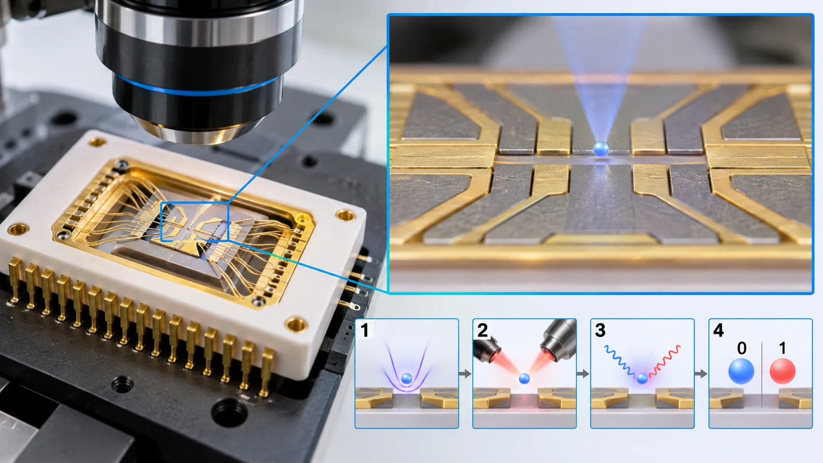
10. Where things stand (checked 16 October 2026) and plans
(1) Quantinuum Helios (a peer-reviewed paper by a company research team)
Helios is a QCCD machine using 98 barium ions as qubits, with all qubits fully connected (any two can be gated directly). Averaged over all zones it reports infidelities of 2.5(1)×10⁻⁵ for one-qubit gates, 7.9(2)×10⁻⁴ for two-qubit gates and 4.8(6)×10⁻⁴ for state preparation and measurement. The authors state that random-circuit sampling shows the machine operating beyond the reach of classical simulation (the authors' claim)[Ref. 2]Sourced. The paper was published in Nature on 17 June 2026[Ref. 2]Sourced. We could not confirm a reproduction of the same performance by another laboratory.
(2) The earlier generation and the move to electrical control
H2, reported by Moses et al. in 2023 (a race-track trap, initially 32 qubits), had an average state-preparation-and-measurement infidelity of 1.6(1)×10⁻³, one-qubit-gate infidelity of 2.5(3)×10⁻⁵ and two-qubit-gate infidelity of 1.84(5)×10⁻³, and measured a quantum volume of QV = 2¹⁶[Ref. 37]Sourced. As seen in Chapter 8, the Oxford Ionics and IonQ team reported control by electrical signals and two-qubit gates without cooling to the ground state (a preprint and a company blog)[Ref. 6, 34, 7]Sourced.
(3) Plans (not yet confirmed)
In its official blog, IonQ mentions a roadmap toward millions of qubits by 2030 and 256-qubit systems scheduled for demonstration in 2026 (a company plan)[Ref. 7]Not yet confirmed. As of the check date we could not confirm an official announcement that a 256-qubit machine was completed, nor the progress of other companies' plans. For any planned number, check whether it counts physical or logical qubits and under what error-rate conditions.
11. Limits, what we could not confirm, and a summary
(1) Full texts of standards
We did not read the full text of ISO/IEC 4879:2024, which is paid. For IEEE P7130 and P7131 we could not retrieve the IEEE pages and confirmed only the existence of the projects through StandICT.eu.
(2) Company claims
IonQ's 99.99% is a company blog claim based on an "estimated" value in an arXiv paper. The Helios result is in a peer-reviewed paper, but we have not confirmed reproduction by other laboratories.
(3) Date of the review
The review by Bruzewicz et al. is from 2019, and the "best values" and "fastest gates" it cites may have been surpassed since. We supplement it with 2023–2026 papers where possible.
(4) Approaches not covered
We do not cover Penning traps, molecular ions, the detailed operation of optical qubits, or networking (photon links between ions).
(5) Progress on plans
Progress on plans such as IonQ's 256-qubit machine is stated only as far as official reports of achievement could be confirmed.
- A trapped-ion machine uses a single atomic ion floated by electric fields as the qubit. 0 and 1 are two internal states of the atomSourced
- Ions of one species are all identical and precision is high — but errors are not zeroSourced
- Control is by laser light (or microwaves or electrical signals). Two-qubit gates use the ions' shared motion as a go-between. About 70 μs, an example roughly a thousand times slower than superconductingSourcedOur calculation
- Readout is the fluorescence "bright or dark." Under 1 ms in some examplesSourced
- Scaling relies on the QCCD that moves ions, optics built into the chip, and control by electrical signals. Surface noise of electrodes, vacuum, magnetic field and optics are the challenges for materials engineersSourced
12. How to read evaluations and standards
A trapped-ion machine's performance is read through gate error rates (one- and two-qubit), state-preparation and measurement errors, state-holding time and the quality of the whole machine. High precision is its hallmark, but each number changes with "which pair, averaged over what, measured how." For standards, vocabulary has come first, while standards for how to measure performance are still at the project stage (checked 16 October 2026).
| What is evaluated | Representative benchmarks and evaluation methods (name, source) | Standards and guidance (NIST, ISO/IEC, IEEE, ETSI, ITU-T, IETF, etc.) | Cautions in reading |
|---|---|---|---|
| Gate accuracy (one- and two-qubit) | Report the average infidelity of gates by randomized benchmarking (RB). Example: Helios two-qubit gate 7.9(2)×10⁻⁴ (average over all zones)[Ref. 2, 38]Sourced. Ballance et al. report 99.9(1)% over gate times of 3.8–520 μs[Ref. 8]Sourced | We could not confirm one | Check whether it is for one pair or an average over all pairs, and how long the gate takes (the number is conditional) |
| State preparation and measurement (SPAM) | The average infidelity of preparation and measurement together. Helios: 4.8(6)×10⁻⁴; H2: 1.6(1)×10⁻³[Ref. 2, 37]Sourced | We could not confirm one | The number changes with where the detection threshold is set and over how many ions it is averaged |
| State-holding time | Report the coherence time (T2 and the like) with how it was measured (Ramsey, echo, dynamical decoupling). Example: up to 600 s with 171Yb⁺ (dynamical decoupling)[Ref. 1]Sourced. Over an hour is an "estimate"[Ref. 10]Sourced | We could not confirm one | A value with dynamical decoupling and one without are different things. Do not rank them against values of other kinds of qubits |
| Quality of the whole machine | Quantum volume: QV = 2¹⁶ for H2; mirror benchmarking; linear cross-entropy benchmarking[Ref. 37, 39]Sourced | We could not confirm one | QV is a discrete value expressed as a power of two. It does not necessarily reflect the quality of machines with many qubits (the Helios paper also uses random-circuit sampling) |
| Plans versus achievements | IonQ's roadmap (256-qubit systems scheduled for demonstration in 2026, and so on). A statement in a company blog[Ref. 7]Not yet confirmed | We could not confirm one | A goal is not an achieved fact. Check whether the figure is physical or logical |
| Is the physical system a good raw material for a quantum computer? | DiVincenzo's seven items (five requirements plus two on communication): (1) many well-characterized qubits, (2) initialization, (3) coherence time much longer than a gate, (4) a universal set of gates, (5) qubit-specific measurement, (6)(7) two items on communication[Ref. 41]Sourced | We could not confirm one (this is a paper's framework, not a standard) | It is a checklist, not a score. Each of the four approaches meets the items in different ways and has different weak points |
| Gate accuracy (one- and two-qubit) | Randomized benchmarking (RB): run random gate sequences and infer the average error from how success decays (Knill et al., 2008; Magesan et al., 2011)[Ref. 42, 38]Sourced | IEEE P7131 (quantum computing performance metrics and benchmarking) is at the project stage[Ref. 43]Not yet confirmed | Read "99.9% fidelity" together with which operation was measured and how. RB numbers depend on how the test is done |
| Quality of the whole machine | Quantum volume (Cross et al., 2019), EPLG (McKay et al., 2023), CLOPS (Wack et al., 2021), a method to measure capabilities (Proctor et al., 2022)[Ref. 39, 27, 44, 45]Sourced | We could not confirm one (IEEE P7131 is at the project stage)[Ref. 43]Not yet confirmed | Each metric measures something different. Do not decide a machine's merit from one number (a survey of benchmarks: Acuaviva et al., 2026[Ref. 46]) |
| Terminology and definitions | — (a vocabulary standard, not an evaluation method) | ISO/IEC 4879:2024 "Information technology — Quantum computing — Vocabulary" (first edition, May 2024, published)[Ref. 40]Sourced. IEEE P7130 (quantum technology definitions) is at the project stage[Ref. 47]Not yet confirmed | The standards' full texts are paid, so we did not read them. We do not state their requirements or definitions |
The arrangement of the table is Our calculation (organization). Because the standards' full texts are paid, we give only titles and status (checked 16 October 2026).
Cautions in reading (for materials engineers)
- "How many qubits" alone does not tell performance. In ions, lengthening a row slows gates, and the time to move ions in a QCCD is added[Ref. 1, 2]
- Check average versus best, one pair versus all pairs. Helios's 7.9×10⁻⁴ is an average over all zones; Ballance et al.'s 99.9% is a conditional value for one pair[Ref. 2, 8]
- A company's announcement and third-party verification are different. IonQ's 99.99% is the company's claim based on an "estimated" value; we have not confirmed a reproduction by another laboratory[Ref. 34, 7]
- Check whether a standard is a recommendation or a requirement, and whether it is legally binding. ISO/IEC 4879 is a vocabulary standard and does not guarantee performance[Ref. 40]. Plans are Not yet confirmed
13. Glossary
- Qubit
- The unit of information in a quantum computer. It can point in a direction between 0 and 1. In the series' shared picture, an "arrow."
- Ion
- An atom with electrons removed so it carries charge. Electric fields can hold it in mid-air.
- Paul trap
- A device that floats ions with an electric field whose direction is swapped very fast.
- Earnshaw's theorem
- The theorem that static electric forces alone cannot stably confine a charge in all three directions.
- RF (radio frequency)
- Flipping the field direction tens of millions of times per second.
- Laser cooling
- A method that uses the absorption and emission of light to slow an ion's motion.
- Doppler limit
- The lower limit of temperature reached by the first stage of laser cooling: a few hundred μK.
- Hyperfine levels
- Two steps of very close energy within an atom's ground state; the gap is about a GHz.
- Clock state
- A pair of states insensitive to magnetic field, which hold their state for a long time.
- Raman transition
- A way to move between 0 and 1 using a frequency equal to the difference between two laser beams.
- Shared motion (motional mode)
- The motion in which the whole row of ions sways together; the go-between of two-qubit gates.
- Mølmer–Sørensen gate
- A two-qubit gate that uses the shared motion; it works even with leftover thermal motion.
- Fluorescence
- The phenomenon in which an atom that has absorbed light re-emits it. Bright / dark gives 0 and 1.
- SPAM
- State Preparation And Measurement: a metric combining preparation and measurement errors.
- QCCD
- A scaling approach that moves ions between logic and memory zones (quantum charge-coupled device).
- Junction
- A crossroads on the trap that routes ions to where they need to go.
- Sympathetic cooling
- Mixing in a second ion species and cooling it so that it draws heat from the qubit ions.
- Anomalous heating
- An ion heating up by itself because of electric-field noise from the electrode surface.
- Ion milling
- A treatment that scrapes a surface with ions to remove contamination.
- Waveguide / grating coupler
- A part that makes a light path inside a chip, and a part that directs light out of the chip.
- Randomized benchmarking (RB)
- A method that runs random gate sequences and infers the average error from how success decays.
- Quantum volume (QV)
- A metric that expresses a machine's overall quality in one number (a power of two).
14. References (primary sources)
- Bruzewicz C. D. et al. "Trapped-ion quantum computing: Progress and challenges", Appl. Phys. Rev. 6, 021314 (2019), DOI 10.1063/1.5088164 — doi.org/10.1063/1.5088164
- Ransford A. et al. (Quantinuum) "A 98-qubit trapped-ion quantum computer with all-to-all connectivity", Nature 655, 81–86 (2026), DOI 10.1038/s41586-026-10676-4 (we read the preprint arXiv:2511.05465 "Helios: A 98-qubit trapped-ion quantum computer") — doi.org/10.1038/s41586-026-10676-4
- Kielpinski D., Monroe C., Wineland D. J. "Architecture for a large-scale ion-trap quantum computer", Nature 417, 709–711 (2002), DOI 10.1038/nature00784 — doi.org/10.1038/nature00784
- Pino J. M. et al. "Demonstration of the trapped-ion quantum CCD computer architecture", Nature 592, 209–213 (2021), DOI 10.1038/s41586-021-03318-4 — doi.org/10.1038/s41586-021-03318-4
- Mehta K. K. et al. "Integrated optical multi-ion quantum logic", Nature 586, 533–537 (2020), DOI 10.1038/s41586-020-2823-6 — doi.org/10.1038/s41586-020-2823-6
- Löschnauer C. M. et al. (Oxford Ionics) "Scalable, high-fidelity all-electronic control of trapped-ion qubits", PRX Quantum 6, 040313 (2025), DOI 10.1103/h4wk-v31j — doi.org/10.1103/h4wk-v31j
- IonQ "Accelerating Towards Fault Tolerance: Unlocking 99.99% Two-Qubit Gate Fidelities" (company blog, 21 October 2025) — ionq.com/blog/accelerating-towards-fault-tolerance-unlocking-99-99-two-qubit-gate
- Ballance C. J. et al. "High-fidelity quantum logic gates using trapped-ion hyperfine qubits", Phys. Rev. Lett. 117, 060504 (2016), DOI 10.1103/PhysRevLett.117.060504 — doi.org/10.1103/PhysRevLett.117.060504
- Gaebler J. P. et al. "High-fidelity universal gate set for 9Be+ ion qubits", Phys. Rev. Lett. 117, 060505 (2016), DOI 10.1103/PhysRevLett.117.060505 — doi.org/10.1103/PhysRevLett.117.060505
- Wang P. et al. "Single ion qubit with estimated coherence time exceeding one hour", Nat. Commun. 12, 233 (2021), DOI 10.1038/s41467-020-20330-w — doi.org/10.1038/s41467-020-20330-w
- Cirac J. I., Zoller P. "Quantum computations with cold trapped ions", Phys. Rev. Lett. 74, 4091–4094 (1995), DOI 10.1103/PhysRevLett.74.4091 — doi.org/10.1103/PhysRevLett.74.4091
- Sørensen A., Mølmer K. "Quantum computation with ions in thermal motion", Phys. Rev. Lett. 82, 1971–1974 (1999), DOI 10.1103/PhysRevLett.82.1971 — doi.org/10.1103/PhysRevLett.82.1971
- Krantz P. et al. "A quantum engineer's guide to superconducting qubits", Appl. Phys. Rev. 6, 021318 (2019), DOI 10.1063/1.5089550 — doi.org/10.1063/1.5089550
- Evered S. J. et al. "High-fidelity parallel entangling gates on a neutral-atom quantum computer", Nature 622, 268–272 (2023), DOI 10.1038/s41586-023-06481-y (we also read the arXiv:2304.05420 version) — doi.org/10.1038/s41586-023-06481-y
- Ma S. et al. "High-fidelity gates and mid-circuit erasure conversion in an atomic qubit", Nature 622, 279–284 (2023), DOI 10.1038/s41586-023-06438-1 — doi.org/10.1038/s41586-023-06438-1
- Radnaev A. G. et al. (Infleqtion) "A universal neutral-atom quantum computer with individual optical addressing and non-destructive readout", PRX Quantum 6, 030334 (2025), DOI 10.1103/66s8-jj18 — doi.org/10.1103/66s8-jj18
- Alexander K. et al. (PsiQuantum) "A manufacturable platform for photonic quantum computing", Nature 641, 876–883 (2025), DOI 10.1038/s41586-025-08820-7 (we also read the arXiv:2404.17570 version) — doi.org/10.1038/s41586-025-08820-7
- Aghaee Rad J. et al. (Xanadu) "Scaling and networking a modular photonic quantum computer", Nature 638, 912–919 (2025), DOI 10.1038/s41586-024-08406-9 — doi.org/10.1038/s41586-024-08406-9
- Kok P. et al. "Linear optical quantum computing with photonic qubits", Rev. Mod. Phys. 79, 135–174 (2007), DOI 10.1103/RevModPhys.79.135 — doi.org/10.1103/RevModPhys.79.135
- IBM "IBM Quantum — Technology" (official page; checked 16 October 2026) — www.ibm.com/quantum/technology
- Saffman M., Walker T. G., Mølmer K. "Quantum information with Rydberg atoms", Rev. Mod. Phys. 82, 2313–2363 (2010), DOI 10.1103/RevModPhys.82.2313 — doi.org/10.1103/RevModPhys.82.2313
- Bartolucci S. et al. (PsiQuantum) "Fusion-based quantum computation", Nat. Commun. 14, 912 (2023), DOI 10.1038/s41467-023-36493-1 — doi.org/10.1038/s41467-023-36493-1
- Blais A. et al. "Circuit quantum electrodynamics", Rev. Mod. Phys. 93, 025005 (2021), DOI 10.1103/RevModPhys.93.025005 — doi.org/10.1103/RevModPhys.93.025005
- Wallraff A. et al. "Strong coupling of a single photon to a superconducting qubit using circuit quantum electrodynamics", Nature 431, 162–167 (2004), DOI 10.1038/nature02851 — doi.org/10.1038/nature02851
- Manetsch H. J. et al. "A tweezer array with 6,100 highly coherent atomic qubits", Nature 647, 60–67 (2025), DOI 10.1038/s41586-025-09641-4 (we read the abstract of the arXiv:2403.12021 version) — doi.org/10.1038/s41586-025-09641-4
- Bluvstein D. et al. "A fault-tolerant neutral-atom architecture for universal quantum computation", Nature 649, 39–46 (2025), DOI 10.1038/s41586-025-09848-5 (we read the abstract of the arXiv:2506.20661 version) — doi.org/10.1038/s41586-025-09848-5
- McKay D. C. et al. "Benchmarking quantum processor performance at scale", arXiv:2311.05933 (preprint, November 2023) — arxiv.org/abs/2311.05933
- Bluvstein D. et al. "A quantum processor based on coherent transport of entangled atom arrays", Nature 604, 451–456 (2022), DOI 10.1038/s41586-022-04592-6 — doi.org/10.1038/s41586-022-04592-6
- Google Quantum AI, Acharya R. et al. "Quantum error correction below the surface code threshold", Nature 638, 920–926 (2025), DOI 10.1038/s41586-024-08449-y (we also read the arXiv:2408.13687 version) — doi.org/10.1038/s41586-024-08449-y
- Bland M. P. et al. "Millisecond lifetimes and coherence times in 2D transmon qubits", Nature 647, 343–348 (2025), DOI 10.1038/s41586-025-09687-4 (we also read the arXiv:2503.14798 version) — doi.org/10.1038/s41586-025-09687-4
- Krinner S. et al. "Engineering cryogenic setups for 100-qubit scale superconducting circuit systems", EPJ Quantum Technol. 6, 2 (2019), DOI 10.1140/epjqt/s40507-019-0072-0 — doi.org/10.1140/epjqt/s40507-019-0072-0
- Zhang E. J. et al. "High-fidelity superconducting quantum processors via laser-annealing of transmon qubits", arXiv:2012.08475 (published as Sci. Adv. 8, eabi6690 (2022); we read the abstract of the arXiv version) — arxiv.org/abs/2012.08475
- Chiu N.-C. et al. "Continuous operation of a coherent 3,000-qubit system", Nature 646, 1075–1080 (2025), DOI 10.1038/s41586-025-09596-6 — doi.org/10.1038/s41586-025-09596-6
- Hughes A. C. et al. "Trapped-ion two-qubit gates with >99.99% fidelity without ground-state cooling", arXiv:2510.17286 (preprint, October 2025) — arxiv.org/abs/2510.17286
- Brownnutt M. et al. "Ion-trap measurements of electric-field noise near surfaces", Rev. Mod. Phys. 87, 1419–1482 (2015), DOI 10.1103/RevModPhys.87.1419 — doi.org/10.1103/RevModPhys.87.1419
- Niffenegger R. J. et al. "Integrated multi-wavelength control of an ion qubit", Nature 586, 538–542 (2020), DOI 10.1038/s41586-020-2811-x — doi.org/10.1038/s41586-020-2811-x
- Moses S. A. et al. "A race-track trapped-ion quantum processor", Phys. Rev. X 13, 041052 (2023), DOI 10.1103/PhysRevX.13.041052 — doi.org/10.1103/PhysRevX.13.041052
- Magesan E., Gambetta J. M., Emerson J. "Scalable and robust randomized benchmarking of quantum processes", Phys. Rev. Lett. 106, 180504 (2011), DOI 10.1103/PhysRevLett.106.180504 — doi.org/10.1103/PhysRevLett.106.180504
- Cross A. W. et al. "Validating quantum computers using randomized model circuits", Phys. Rev. A 100, 032328 (2019), DOI 10.1103/PhysRevA.100.032328 — doi.org/10.1103/PhysRevA.100.032328
- ISO/IEC "ISO/IEC 4879:2024 Information technology — Quantum computing — Vocabulary" (ISO page; first edition, May 2024, published) — www.iso.org/standard/80432.html
- DiVincenzo D. P. "The physical implementation of quantum computation", Fortschr. Phys. 48, 771–783 (2000), arXiv:quant-ph/0002077 — arxiv.org/abs/quant-ph/0002077
- Knill E. et al. "Randomized benchmarking of quantum gates", Phys. Rev. A 77, 012307 (2008), DOI 10.1103/PhysRevA.77.012307 — doi.org/10.1103/PhysRevA.77.012307
- StandICT.eu "P7131 - Standard for Quantum Computing Performance Metrics & Performance Benchmarking" (an IEEE project, as listed in the StandICT.eu standards repository; the IEEE page itself could not be retrieved) — standict.eu/standards-repository/p7131-standard-quantum-computing-performance-metrics-performance-benchmarking
- Wack A. et al. "Quality, speed, and scale: three key attributes to measure the performance of near-term quantum computers", arXiv:2110.14108 (preprint, October 2021) — arxiv.org/abs/2110.14108
- Proctor T. et al. "Measuring the capabilities of quantum computers", Nat. Phys. 18, 75–79 (2022), DOI 10.1038/s41567-021-01409-7 — doi.org/10.1038/s41567-021-01409-7
- Acuaviva A. et al. "Benchmarking quantum computers: towards a standard performance evaluation approach", Quantum Sci. Technol. 11, 025004 (2026), DOI 10.1088/2058-9565/ae4269 — doi.org/10.1088/2058-9565/ae4269
- StandICT.eu "P7130 - Standard for Quantum Technologies Definitions" (an IEEE project, as listed in the StandICT.eu standards repository; the IEEE page itself could not be retrieved) — standict.eu/standards-repository/p7130-standard-quantum-technologies-definitions
15. Claim-to-source audit
| Claim in the text | Basis | Type |
|---|---|---|
| Characteristics of trapped ions (trap types; electrode distance 30 μm–1 mm; RF 10–1,000 V at 10–100 MHz; holding time hours to months; hyperfine gap about a GHz; microwave and Raman transitions; all ions identical; readout under 1 ms; efficiency 2–4%; SNSPD about 0.8; fastest gate 1.6 μs and sub-μs gates at or below 76%; longer rows slow gates; clock states from seconds to 600 s; 300 ms and 2.1 s; substrates (sapphire, quartz, silicon), 12 inches, tiling; anomalous heating cut by two orders (about 4 K); surface treatments; 40–80 μm) | Text of the review by Bruzewicz et al. (2019) Reference 1 https://doi.org/10.1063/1.5088164 | Sourced |
| The proposal of two-qubit gates (Cirac and Zoller, 1995), the Mølmer–Sørensen gate (1999), and the proposal (2002) and demonstration (2021) of the QCCD | Bibliographic records and abstracts Reference 11 https://doi.org/10.1103/PhysRevLett.74.4091 Reference 12 https://doi.org/10.1103/PhysRevLett.82.1971 Reference 3 https://doi.org/10.1038/nature00784 Reference 4 https://doi.org/10.1038/s41586-021-03318-4 | Sourced |
| Ballance et al.: two-qubit 99.9(1)%, one-qubit 99.9934(3)%, 43Ca⁺, room-temperature trap, gate times 3.8–520 μs. Gaebler et al.: one-qubit error 3.8×10⁻⁵, two-qubit 8(4)×10⁻⁴, memory coherence over 1 s. Wang et al.: over an hour (estimated) | Abstracts of each paper Reference 8 https://doi.org/10.1103/PhysRevLett.117.060504 Reference 9 https://doi.org/10.1103/PhysRevLett.117.060505 Reference 10 https://doi.org/10.1038/s41467-020-20330-w | Sourced |
| Helios: 98 qubits, 137Ba⁺, X junction, 8 zones and up to 16 qubits, sympathetic cooling with 171Yb⁺ (369 nm), about 70 μs and about 300 μs, average infidelities (2.5×10⁻⁵, 7.9×10⁻⁴, 4.8×10⁻⁴), electrodes and signals in Table I, publication in Nature (17 June 2026) | Text of the Helios preprint (arXiv:2511.05465) and the Nature bibliographic record Reference 2 https://doi.org/10.1038/s41586-026-10676-4 | Sourced |
| H2: average infidelities (SPAM 1.6×10⁻³, one-qubit 2.5×10⁻⁵, two-qubit 1.84×10⁻³), QV = 2¹⁶, initially 32 qubits | Abstract of Moses et al. Reference 37 https://doi.org/10.1103/PhysRevX.13.041052 | Sourced |
| Electrical-signal control (seven zones, up to 10 qubits, one-qubit 99.99916(7)%, two-qubit maximally entangled state 99.97(1)%); the estimated error of 8.4(7)×10⁻⁵ for two-qubit gates without ground-state cooling (preprint) | Abstracts of each paper Reference 6 https://doi.org/10.1103/h4wk-v31j Reference 34 https://arxiv.org/abs/2510.17286 | Sourced |
| IonQ's company blog: the claim of 99.99% (estimated); the Doppler limit of a few hundred μK; 256-qubit systems scheduled for demonstration in 2026; a roadmap to millions of qubits by 2030 (company plans) | IonQ company blog (21 October 2025) Reference 7 https://ionq.com/blog/accelerating-towards-fault-tolerance-unlocking-99-99-two-qubit-gate | Not yet confirmed |
| Mehta et al.: high-fidelity gates on several ions with optical fibers connected directly to a cooled trap. Niffenegger et al.: all wavelengths for Sr⁺ delivered by waveguides (CMOS-compatible). Brownnutt et al.: a survey of electric-field noise | Abstracts of each paper Reference 5 https://doi.org/10.1038/s41586-020-2823-6 Reference 36 https://doi.org/10.1038/s41586-020-2811-x Reference 35 https://doi.org/10.1103/RevModPhys.87.1419 | Sourced |
| DiVincenzo's framework of five requirements (plus two on communication) | Abstract and text of DiVincenzo (2000) Reference 41 https://arxiv.org/abs/quant-ph/0002077 | Sourced |
| Existence and titles of the original randomized-benchmarking papers (Knill et al.; Magesan et al.) | Bibliographic records (checked via Crossref / the publisher's page) Reference 42 https://doi.org/10.1103/PhysRevA.77.012307 Reference 38 https://doi.org/10.1103/PhysRevLett.106.180504 | Sourced |
| Titles and abstracts of the papers on quantum volume, EPLG, CLOPS, capability measurement and the benchmarking survey | Abstracts of each paper Reference 39 https://doi.org/10.1103/PhysRevA.100.032328 Reference 27 https://arxiv.org/abs/2311.05933 Reference 44 https://arxiv.org/abs/2110.14108 Reference 45 https://doi.org/10.1038/s41567-021-01409-7 Reference 46 https://doi.org/10.1088/2058-9565/ae4269 | Sourced |
| Number, title and publication date of ISO/IEC 4879:2024 (first edition, May 2024, published) | ISO page Reference 40 https://www.iso.org/standard/80432.html | Sourced |
| IEEE P7130 and P7131 exist as IEEE projects (we treat their status as project stage and do not call them settled standards) | Listing in the StandICT.eu standards repository (the IEEE page itself could not be retrieved) Reference 47 https://standict.eu/standards-repository/p7130-standard-quantum-technologies-definitions Reference 43 https://standict.eu/standards-repository/p7131-standard-quantum-computing-performance-metrics-performance-benchmarking | Not yet confirmed |
| Facts on other approaches (the four-approach table): the review by Krantz et al., Evered et al., Manetsch et al., Alexander et al., Aghaee Rad et al., and others | Abstracts and texts of each paper Reference 13 https://doi.org/10.1063/1.5089550 Reference 29 https://doi.org/10.1038/s41586-024-08449-y Reference 30 https://doi.org/10.1038/s41586-025-09687-4 Reference 31 https://doi.org/10.1140/epjqt/s40507-019-0072-0 Reference 32 https://arxiv.org/abs/2012.08475 Reference 20 https://www.ibm.com/quantum/technology Reference 14 https://doi.org/10.1038/s41586-023-06481-y Reference 15 https://doi.org/10.1038/s41586-023-06438-1 Reference 16 https://doi.org/10.1103/66s8-jj18 Reference 21 https://doi.org/10.1103/RevModPhys.82.2313 Reference 25 https://doi.org/10.1038/s41586-025-09641-4 Reference 28 https://doi.org/10.1038/s41586-022-04592-6 Reference 26 https://doi.org/10.1038/s41586-025-09848-5 Reference 33 https://doi.org/10.1038/s41586-025-09596-6 Reference 17 https://doi.org/10.1038/s41586-025-08820-7 Reference 18 https://doi.org/10.1038/s41586-024-08406-9 Reference 19 https://doi.org/10.1103/RevModPhys.79.135 Reference 22 https://doi.org/10.1038/s41467-023-36493-1 Reference 23 https://doi.org/10.1103/RevModPhys.93.025005 Reference 24 https://doi.org/10.1038/nature02851 Reference 27 https://arxiv.org/abs/2311.05933 | Sourced |
| The readout calculation example (means of 12 and 0.5, threshold 3, errors of 1.4% and 0.05%); the ratio of gate times (70 μs ÷ 70 ns = 1,000 times); the comparison of signals per qubit | Our calculation (Python; Poisson distributions; inputs are assumptions or the sourced numbers above) | Our calculation |
| Explanations, analogies and the materials engineer's views such as "shaking the field makes it float," the saddle analogy, "the ion is a sensitive surface sensor," and materials issues of vacuum, magnetic field and optics, plus the "In three lines" and "common misconception" boxes | This article's organization and commentary based on published content (our own explanation). Not views expressed by the institutions concerned | Commentary |
| Figures 1 and 12 being ImageGen-generated conceptual illustrations; the other figures being drawings made to explain, not observations of real data | A note in this article (our own) | Commentary |
| Not confirmed: the full texts of ISO/IEC and IEEE standards, the IEEE official pages, reproductions of the Helios and IonQ results by other laboratories, completion of IonQ's 256-qubit machine, and updates to the 2019 review | Could not be confirmed in the primary sources accessible within this study, so not stated (our own) | Commentary |
Last updated: 16 October 2026. Sources are limited to primary ones (peer-reviewed papers, arXiv papers, ISO's official page, and a company blog treated as the company's claim). The standards' full texts are paid and were not read. The readout numerical example is our own assumed calculation, not the performance of any real machine. We could not confirm reproductions by other laboratories, the IEEE official pages, or completion of IonQ's 256-qubit machine, so we do not state them. All figures are explanatory concept diagrams or drawings that include our own calculations; Figures 1 and 12 are ImageGen-generated conceptual illustrations.