TECHNOLOGY EXPLAINER
How to Read Claims of Quantum Advantage
Look at who claims it, on which task, and against what
"A quantum computer did in 200 seconds what would take the world's fastest supercomputer 10,000 years." How should such announcements be read? This article explains the difference between "quantum supremacy", "quantum advantage" and "quantum utility", and how the two standard tasks, random circuit sampling and boson sampling, work, using figures and small numerical examples. It then lines up how classical researchers re-evaluated these claims by finding faster methods, keeping company claims and third-party checks apart, and gives six questions for reading a claim.
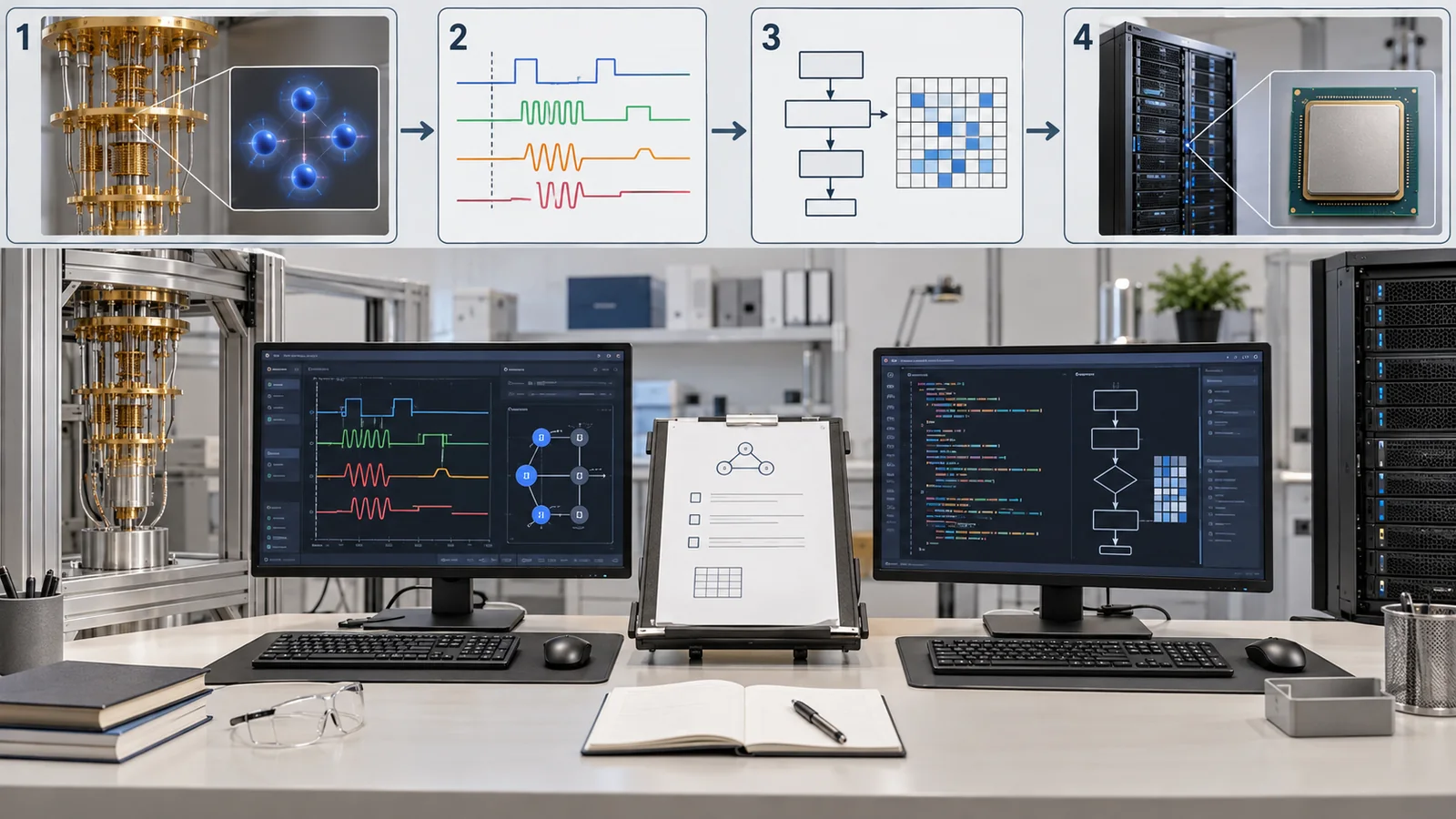
- The short version, what to know first, and where this fits in the series
- Three terms: supremacy, advantage and utility
- Six questions for reading a claim: who, on which task, against what
- Random circuit sampling: how it works, and the XEB yardstick
- Boson sampling: probability distributions made by photon interference
- How classical re-evaluation unfolded: a timeline, and why it happens
- Can the result be checked? Three levels of verifiability
- Advantage is not usefulness: the distance to practical value
- Limits, what we could not confirm, and a summary
- How to read evaluations and standards
- Glossary
- References
- Claim-to-source audit
Sourced = stated in a published source (linked)
Our calculation = a value computed in this article from the stated assumptions
Not yet confirmed = plans, targets, drafts, work in progress, outlooks: not settled
Our own reading for materials engineers is marked as commentary. Inference is shown in bold. Company announcements are labelled as company claims.
1. The short version, what to know first, and where this fits in the series
- "Quantum advantage" means nothing until you ask who claims it, on which task, and against what. Even for one task, the answer changes depending on whether the comparison is "brute force" or "the best known classical algorithm" Sourced[Ref. 11]
- Many of the best-known claims (Google's random circuit sampling, photonic experiments in China and others) were followed by papers in which classical researchers showed faster methods. A re-evaluation, however, does not always use the same conditions or task Sourced[Refs. 4, 5, 12]
- This article does not hand down a verdict. Its aim is to let you read new announcements yourself with six questions (chapter 3). Company announcements are labelled as company claims.
We use the picture of a qubit state as an arrow (north pole = 0, south pole = 1, in between = superposition) that settles on 0 or 1 when measured. Our explainer "Quantum Computing Fundamentals" has the details. This article is readable on its own; it explains what is needed as it goes.
"Classical computer" means an ordinary computer, supercomputers included. "Sampling" means running something many times to collect results (strings of 0s and 1s) that are decided by probability.
A good order is Quantum Algorithms → NISQ and Hybrid Computing → this article. The IBM 127-qubit experiment is explained in the NISQ explainer, D-Wave's claims in the quantum annealing explainer, chemistry and materials in the quantum chemistry explainer, and industrial usefulness in the industrial applications explainer.
2. Three terms: supremacy, advantage and utility
First, three similar-sounding terms. Each paper uses them slightly differently, so the starting point is to check who is using the word, and in what sense.
| Term | Origin and meaning (as the papers state) | Caution |
|---|---|---|
| Quantum supremacy | A term used by Preskill in a 2012 paper, in the context of controlled quantum systems performing tasks beyond what can be done in the classical world [Ref. 1]. Google's 2019 paper presented its 200-second computation as an experimental realization of quantum supremacy for that specific task [Ref. 2] | Does not mean "beats classical at everything"; it concerns one specific task |
| Quantum (computational) advantage | A term common in recent paper titles (Zhong et al. 2020, Madsen et al. 2022, Gao et al. 2025). Madsen et al. define it as outperforming the best classical computers running the best-known algorithms on well-defined tasks [Refs. 10, 11, 8] | "Best known" only: a later classical method can erase the advantage |
| Quantum utility | The word IBM's Kim et al. used in the title of their 2023 paper ("evidence for the utility of quantum computing before fault tolerance"). The paper says it does not aim at problems with proven speed-ups [Ref. 13] | A different claim from "faster than classical". A company claim |
A summary of the origins of each term ([Refs. 1, 2, 11, 13] and others). Usage differs between papers; we could not find a single uniform definition.
There are also efforts to tidy up the definition itself. A joint proposal including IBM tries to give an operational definition of quantum advantage that is platform-agnostic and empirically verifiable Sourced[Ref. 25] (a preprint). An IBM article describes advantage as showing, in a way that can be rigorously validated, that a quantum method is faster, more accurate or more cost-effective than classical-only methods [Ref. 26] (a company's description).
What the papers claim is that, on one specific task (usually chosen because it suits quantum devices, not because it is useful), the machine beat the then-known classical methods. Google's own 2019 paper limits the claim to that specific task Sourced[Ref. 2]. The right reading: an advantage claim is a point, not an area. Whether it carries over to practical tasks has to be checked separately (chapter 8).
3. Six questions for reading a claim: who, on which task, against what
When reading an announcement, check these six questions in order. The cases in the second half of this article are read through them.
| Question | What to check | Example (from the cases in this article) |
|---|---|---|
| 1. Who | Was the claim made by a company or a research group? Has someone else checked it? | Google's 10²⁵-year estimate (a blog post) is a company claim; no third-party re-evaluation was found (chapter 4) |
| 2. On which task | Is the task contrived to suit quantum devices, or useful? | Random circuit sampling has no application (it is a yardstick). Google says its molecule example is "not yet beyond classical" (chapter 8) |
| 3. Against what | Brute-force full-state simulation, or the best known classical algorithm? The classical resources used (cores, time, memory) | Google's 10,000 years was an estimate for the methods of the time; IBM proposed "days" with another method (chapter 4) |
| 4. Under what conditions | Fidelity, error rates, number of samples. A result that is mostly noise can still pass statistically | Sycamore's predicted fidelity was 0.2% (chapter 4); a numerical XEB example is in chapter 4 |
| 5. Verifiable? | Checked directly classically, statistically only, or reproducible on another device? | Chapter 7: three levels |
| 6. What came after | Has classical re-evaluation appeared? Follow it with dates | The timeline in chapter 6, and IBM's advantage tracker (chapter 7) |
The six questions are this article's commentary. See the references at each point in the text for the sources of the examples.
4. Random circuit sampling: how it works, and the XEB yardstick
Random circuit sampling (RCS) means running a randomly built quantum circuit and collecting the 0/1 strings it produces. It is used not to produce a useful answer but as a yardstick for whether a quantum device can create states that are hard for classical computers. Boixo et al. discussed it as a candidate for testing quantum supremacy on noisy near-term devices Sourced[Ref. 3].
(1) XEB: one number for "do likely strings really appear often?"
Whether the device behaves correctly is checked with the linear cross-entropy benchmark (XEB). In the definition of Arute et al., for the bit strings x₁, x₂, … obtained from the device, one computes each string's ideal probability P(xᵢ) on a classical computer and takes the average: FXEB = 2ⁿ ⟨P(xᵢ)⟩ − 1 (n is the number of qubits) Sourced[Ref. 2]. If the strings follow the ideal distribution the value is about 1; if they are completely random it is 0.
Let us check with a small example. Build one random 14-qubit state (seed 7) and draw a million samples from its ideal distribution: XEB comes out at 0.989. Uniform random strings give −0.0005 (about zero). If only 20% of the samples come from the ideal distribution and the rest are random, XEB is 0.197; at 5% it is 0.049. So XEB is roughly proportional to the share of ideal samples Our calculation. In other words, XEB indicates how much of the sample set follows the ideal distribution.
This is the key point. For Google's 53-qubit, 20-cycle circuits, the predicted fidelity, built up from gate and measurement errors, was 0.2%. The circuits contain 1,113 single-qubit gates and 430 two-qubit gates. The paper says this fidelity is resolvable with a few million measurements (the uncertainty of XEB is 1/√samples) Sourced[Ref. 2]. So even if 99.8% is noise-like, the remaining 0.2% "signal" was extracted and confirmed statistically.
- With 10⁵ samples even the sign of a 0.2% signal is unclear (measured −0.0028, standard error 0.003). With 10⁷ samples it reads 0.0019 (standard error 0.0003), finally close to the true 0.002 Our calculation
- Resolving it at 3σ (three standard errors) needs (3 ÷ 0.002)² ≈ 2.25 million samples Our calculation, consistent with Google's "a few million"
- Computing XEB needs the ideal distribution itself, which is a large classical calculation. For large circuits it cannot be done directly, so Arute et al. check simplified circuits and small patches and extrapolate (chapter 7) Sourced[Ref. 2]
The content of the claim is that producing samples of the same fidelity on a classical computer takes an enormous amount of time. Arute et al. also account for the fact that a lower fidelity lets classical methods save work (a 0.1% fidelity cuts the cost by about 1,000) Sourced[Ref. 2]. Conversely, classical researchers can look for methods that exploit the fact that low-fidelity samples are enough. That is the entry point of the next re-evaluation (Pan et al.).
(2) Main RCS claims and classical re-evaluations
| Experiment | Claim (who and what) | Classical re-evaluation | Reading |
|---|---|---|---|
| Google Sycamore (2019) | About a million samples on 53 qubits in about 200 s; classical sampling of equal fidelity would take about 10,000 years on a million cores (Google's estimate) [Ref. 2] | IBM's Pednault et al. proposed "days" on the Summit supercomputer using secondary storage (2019) [Ref. 4]. Pan et al. generated a million samples of fidelity about 0.0037 in about 15 hours on 512 GPUs with a tensor-network method (2022) [Ref. 5] | The classical estimate fell sharply, though the conditions differ (chapter 6) |
| Google Willow (2024) | On a 105-qubit chip, RCS in under five minutes, which a supercomputer would need 10²⁵ years (10 septillion years) for (a claim in Google's blog) [Ref. 7] | Not found | The details behind the estimate (classical resources and conditions) could not be confirmed from the blog |
| Google (Morvan et al. 2024) | RCS on 67 qubits and 32 cycles is beyond existing supercomputers (Google's claim); depending on noise there is a transition between a regime that classical computers can spoof and a complex one [Ref. 6] | Not found | The authors themselves note that there is a regime where high noise lets classical methods reproduce the output |
| USTC Zuchongzhi 3.0 (2025) | 105 qubits. RCS on 83 qubits and 32 cycles gives a million samples in a few hundred seconds; the group estimates about 6.4×10⁹ years on Frontier (the research group's claim). Two-qubit gate fidelity 99.62% [Ref. 8] | Not found | The two-qubit gate fidelity is as stated in the abstract (see the paper for how it was measured) |
A summary of what each paper or blog states. The numbers of years are estimates for the stated classical methods and resources and cannot be compared directly. Checked on 16 October 2026.
5. Boson sampling: probability distributions made by photon interference
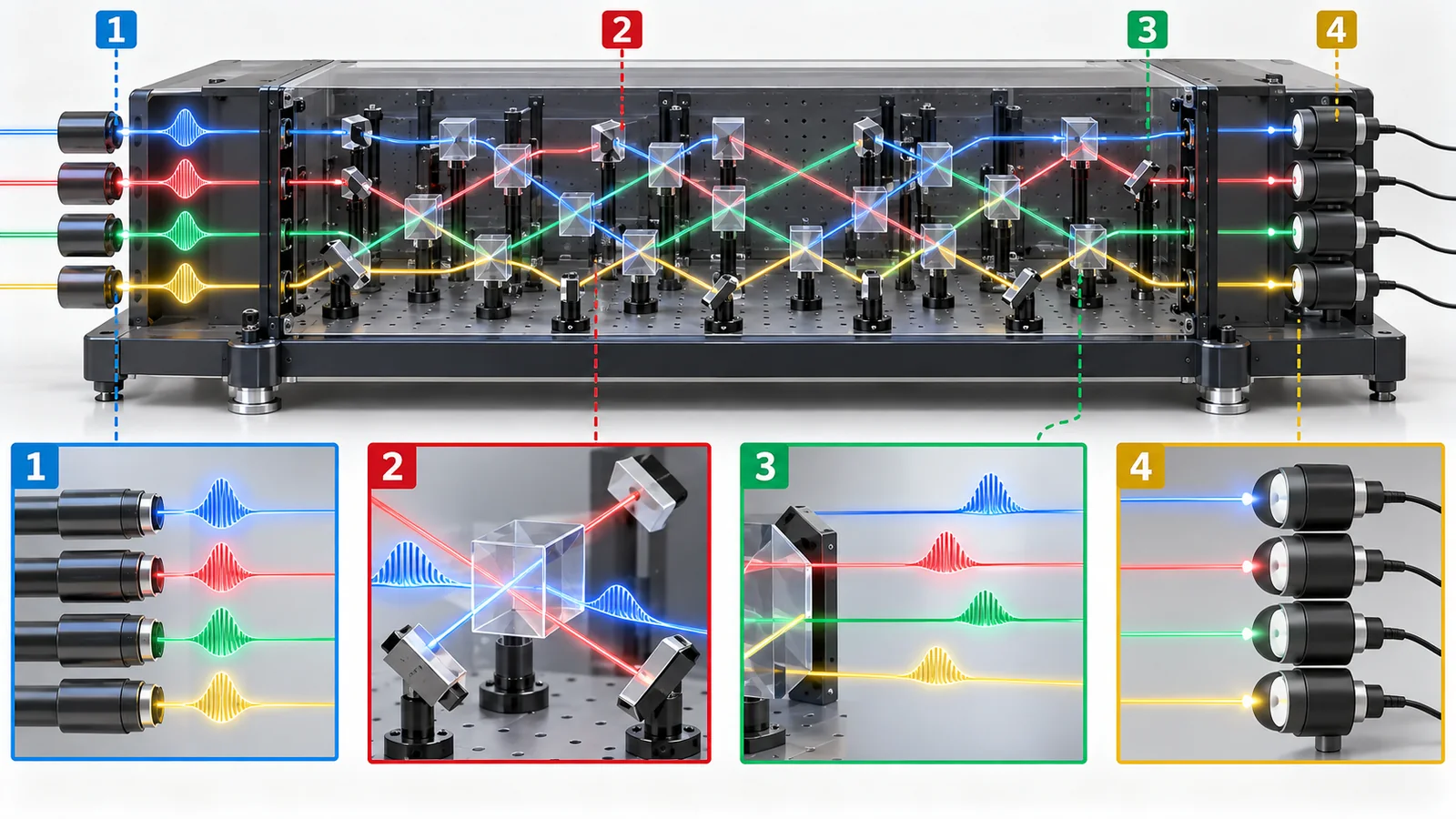
Boson sampling sends photons through an interferometer (a web of light paths) and counts which exits the photons came out of. In 2011 Aaronson and Arkhipov gave a theoretical argument that if a classical computer could efficiently sample from the same distribution as this device, a hierarchy believed in complexity theory would collapse Sourced[Ref. 9] (the argument is for a very accurate device; with noise it rests on assumptions).
View original SVG, values and sources
Original SVG reference: Concept diagram (vector drawing). The flow of Gaussian boson sampling. Squeezed light passes through an interferometer and the click pattern is read at the detectors.
Experiments use the easier-to-realise Gaussian boson sampling (GBS). In 2020, Zhong et al. at USTC fed 50 squeezed-light inputs into a 100-mode interferometer and observed up to 76 clicks. The output state space has size 10³⁰, and they estimate a speed 10¹⁴ times higher than the best classical methods on supercomputers Sourced[Ref. 10] (the research group's claim). In 2022, Xanadu's Madsen et al. observed up to 219 photons in 216 squeezed modes and reported that exact classical methods would need more than 9,000 years per sample while the device takes 36 microseconds Sourced[Ref. 11] (a company claim).
Classical rebuttals followed. In 2024, Oh et al. presented a classical tensor-network algorithm whose cost drops as the photon loss rises, and reported reproducing the largest GBS experiment so far with modest computational resources. The paper says it shows evidence that the classical algorithm matches the ideal distribution better than the experiment does, on the benchmarks the experiments used as evidence of advantage Sourced[Ref. 12]. Madsen et al. themselves noted that earlier photonic experiments were vulnerable to classical approximations (spoofing) Sourced[Ref. 11].
The more photons are lost along the way, the less "quantum entanglement" survives in the output, and the closer the structure comes to something classical computers can approximate (our commentary; Oh et al. describe it as a method that greatly reduces cost when loss is high Sourced[Ref. 12]). The point to take away: a bigger device with high loss may still sit in a regime that classical computers can reproduce.
6. How classical re-evaluation unfolded: a timeline, and why it happens
The cases so far are collected in a timeline of claims and classical re-evaluations, together with IBM's 127-qubit experiment (explained in the NISQ explainer), D-Wave's quantum-simulation claim and Google's Quantum Echoes.
| Claim | Classical re-evaluation (papers) | What the re-evaluation shows, and caveats |
|---|---|---|
| IBM 127 qubits "utility" (2023) | Tindall et al.: a tensor network matched to the lattice (2024) [Ref. 14]. Begušić et al.: sparse Pauli dynamics (2024) [Ref. 15]. Kechedzhi et al. (Google researchers): a framework linking the achievable signal to computational cost through the effective circuit volume (2024) [Ref. 16] | Tindall et al. report a classical simulation more accurate and precise than the quantum processor's results; Begušić et al. report a laptop-core calculation faster than the reported quantum runtime and in good agreement with the zero-noise-extrapolated results |
| D-Wave "beyond-classical" (2025) | King et al.: the annealer rapidly produces samples in close agreement with solutions of the Schrödinger equation, and leading tensor-network and neural-network approximations cannot reach the same accuracy in reasonable time (a company claim) [Ref. 21]. Tindall et al.: lattice-specific tensor networks with belief propagation reach state-of-the-art accuracy with modest resources (Science 2026) [Ref. 22]. Mauron and Carleo: time-dependent variational Monte Carlo reaches comparable accuracy up to 128 spins (preprint) [Ref. 23] | Details in the quantum annealing explainer. The conclusion changes with the classical method compared |
| Google Quantum Echoes (2025) | Google: it measured second-order OTOCs on a superconducting processor and estimated that obtaining the same accuracy classically would take about 13,000 times longer (a company claim). Google says it implemented and costed nine classical simulation methods and spent about ten person-years on red-teaming [Refs. 17, 18]. Bermejo et al. (with Google-affiliated authors): tensor networks with belief propagation cannot feasibly reproduce the experiment (April 2026, preprint) [Ref. 19]. Kshetrimayum et al.: a review from the tensor-network viewpoint (March 2026, preprint) [Ref. 20] | We found no independent classical refutation of this claim. The Bermejo et al. paper includes Google-affiliated authors and concerns one method |
A summary of what each paper states. It does not decide that an advantage "vanished" or "survived". Checked on 16 October 2026.
(1) The classical estimate falling on the same task
Here is how the classical estimate changed for Sycamore. In 2019 Google estimated about 10,000 years; in the same month IBM proposed "days" using Summit and secondary storage; and in 2022 Pan et al. made low-fidelity samples in 15 hours. 10,000 years is about 8.8×10⁷ hours, so the estimate fell by several orders of magnitude Our calculation.
A new classical method does not undo the fact that the quantum experiment pushed beyond the known classical methods of its time. And the faster the classical methods become, the bigger and more accurate the next quantum experiment must be to show an advantage. The exchange of claims and re-evaluations proceeds as a race between the quantum and classical sides (our commentary).
(2) Why re-evaluations happen
- Noise simplifies the state: real samples have less entanglement than the ideal state and are easier to approximate. Kechedzhi et al. related the achievable signal to the classical cost through the effective circuit volume Sourced[Ref. 16]
- The required accuracy is low: when only 0.2% fidelity or a single expectation value is needed, classical methods can skip more work Sourced[Refs. 2, 5]
- Classical methods keep improving: new methods that exploit a task's structure, such as tensor networks and sparse Pauli dynamics, appear, and supercomputers get faster too Sourced[Refs. 14, 15, 5]
7. Can the result be checked? Three levels of verifiability
A central question in advantage claims is how to check that the quantum device's output is correct. There is a catch: a task that is hard for classical computers is also hard to verify classically. Arute et al. say so plainly. For 20-cycle circuits, a million samples take the device 200 s, equal-fidelity classical sampling takes 10,000 years on a million cores, and verifying the fidelity would take millions of years. The largest circuits that can be verified directly have 53 qubits but a simplified gate arrangement Sourced[Ref. 2].
- Level 1: Kim et al. (IBM) first confirmed correctness on circuits that can be verified exactly classically, then moved to circuits beyond classical brute force Sourced[Ref. 13]
- Level 3: For Quantum Echoes, Google explains that expectation values such as current and magnetization are verifiable results that stay the same on different quantum computers, unlike strings of random bits [Ref. 18] (a company claim; the molecular application is in a separate, un-reviewed paper that the same blog says is "not yet beyond classical").
- An example where classical supercomputing is used to verify and make the result valuable: a Quantinuum-led team used the 56-qubit trapped-ion computer H2-1 over the Internet to generate certified randomness, verified with classical supercomputers (combined 1.1×10¹⁸ operations per second); they report certifying 71,313 bits of entropy under a restricted adversary and additional assumptions Sourced[Ref. 24] (a report by a company and collaborators). It turns the classical hardness of random circuits into the task itself.
There are also attempts to follow claims in public. IBM, with the Flatiron Institute, BlueQubit, Algorithmiq and others, started a "quantum advantage tracker" that collects candidates and compares them with the best classical methods (a few months before its February 2026 article). IBM's article says that as of February 2026 the community had not yet reached advantage (it needs rigorous validation and a demonstrable quantum separation), and describes a case from BlueQubit with "peaked circuits" in which a quantum runtime advantage was reversed by new classical methods [Ref. 26] (a company's description).
8. Advantage is not usefulness: the distance to practical value
Random circuit sampling and boson sampling are not tasks whose results lead directly to applications; they are yardsticks. For Quantum Echoes, Google showed in a separate, un-reviewed paper an application that combines OTOC measurements with nuclear magnetic resonance (NMR) data to study molecular structure, but the same blog says "this initial demonstration is not yet beyond classical" [Ref. 18]. So the tasks where advantage was shown and the tasks of useful applications do not yet coincide.
In its Quantum Benchmarking Initiative (QBI), the US agency DARPA defines "utility-scale" as a machine whose computational value exceeds its cost, and acts as a third party checking whether an industrially useful quantum computer can be built by 2033. As of 8 October 2026, two companies participate in Stage A, seven in Stage B and six in Stage C Sourced[Ref. 27]. DARPA estimates it is "more likely than not" that at least one company will build an industrially useful quantum computer by 2033 Not yet confirmed, but this is an estimate and a goal, not an achievement.
The performance of the devices behind advantage claims rests on materials and fabrication. For example, the Zuchongzhi 3.0 paper reports fidelities of 99.90% for single-qubit gates, 99.62% for two-qubit gates and 99.18% for readout Sourced[Ref. 8] (as stated in the abstract; do not rank them against devices of other types). Using the formula from the NISQ explainer, a two-qubit gate error of 0.38% corresponds to a 50% success chance after about 182 gates Our calculation.
For materials engineers, the lesson is that advantage claims rest on a mechanism for extracting a statistical signal from mostly noisy results (chapter 4). If the materials that set the error rate (defects, interfaces, substrate loss) improved by a factor of ten, how "noise-dominated" the results are would change a great deal. Progress in device materials and fabrication directly widens the range of tasks on which advantage can be claimed (our commentary; see our explainers on superconducting qubits and on materials and fabrication).
D-Wave's claim concerns quantum simulation of magnetic materials (the time evolution of spin glasses) Sourced[Ref. 21]. Materials engineers should check three things. (1) Is the task a real material? It is a model (an artificial lattice with spin interactions), not the properties of a specific substance. (2) What was it compared with? It was compared with several classical methods such as tensor networks, and other classical methods have since been reported to reach comparable accuracy (chapter 6). (3) Is the accuracy usable for materials decisions? Agreement on a model does not guarantee a link to measured properties.
Do not use an "advantage" story directly to judge whether a method will help materials research. Applications to chemistry and materials are sorted out, together with the conditions of comparison with the best classical methods, in the quantum chemistry and materials simulation explainer.
9. Limits, what we could not confirm, and a summary
(1) What we could not confirm
- For Google Willow's RCS claim (10²⁵ years) we confirmed only the blog statement and could not confirm the details behind the estimate (classical resources and conditions).
- We found no classical re-evaluation papers for the Willow and Zuchongzhi 3.0 claims (a limit of our search, not proof that none exist).
- We found no independent classical refutation of Quantum Echoes. The two 2026 preprints (Bermejo et al.; Kshetrimayum et al.) are not peer-reviewed.
- The text of ISO/IEC 4879:2024 (quantum computing vocabulary) is paywalled, so we could not confirm whether terms such as "quantum advantage" are defined. IEEE P7131 and similar efforts were confirmed only as working-group activities in development.
- The estimates in the papers (years, factors) are for the stated classical methods and resources and are not like-for-like comparisons.
- Quantum advantage is a claim about a point. Check who, on which task, against what (the six questions) Sourced
- XEB in RCS is a yardstick for extracting a signal of about 0.2% from mostly noisy results (Sycamore's predicted fidelity was 0.2%), requiring millions of samples SourcedOur calculation
- Most of the best-known claims were followed by classical re-evaluation (Sycamore's estimate fell from about 10,000 years to days and then 15 hours; GBS, IBM and D-Wave too), though the conditions are not the same Sourced
- Think of verification in three levels: direct classical, statistical only, or reproducible on another device. Keep company announcements and third-party checks apart Sourced
- Advantage is not the same as usefulness. DARPA's QBI uses "value exceeds cost" as its standard and checks claims as a third party Sourced
10. How to read evaluations and standards
The yardsticks of quantum advantage split into yardsticks for device quality (XEB, quantum volume) and frameworks for checking claims (comparison with classical methods, third-party verification). The first measures how close a device is to the ideal; the second checks whether it beats the best classical methods. Read both with attention to what is and is not measured. Checked on 16 October 2026.
| Item | Representative benchmarks and methods (name, source) | Standards and guidance (ISO/IEC, IEEE, DARPA, etc.) | Reading notes |
|---|---|---|---|
| Is the device close to ideal (RCS) | Linear cross-entropy benchmarking, XEB (Boixo et al. 2018; Arute et al. 2019) [Refs. 3, 2]; noise-driven phase transitions (Morvan et al. 2024) [Ref. 6]Sourced | Not found (we did not find an international standard defining XEB) | XEB needs a classical calculation of the ideal distribution; at large scale it is extrapolated from simplified circuits (chapters 4 and 7) |
| Whole-machine quality | Quantum volume (Cross et al. 2019) [Ref. 28]Sourced | Not found | One number does not decide on which tasks advantage can be claimed |
| Definition of advantage | A proposed operational definition, "A framework for quantum advantage" (Lanes et al. 2025, preprint) [Ref. 25]; the definition in Madsen et al. [Ref. 11]SourcedNot yet confirmed | ISO/IEC 4879:2024 (vocabulary, published May 2024) [Ref. 29]. The text is paywalled; whether it defines advantage is unconfirmedSourced | Definitions differ between papers; we could not find an "official" one |
| Tracking claims | The quantum advantage tracker (IBM, Flatiron, BlueQubit, Algorithmiq; started a few months before the article of February 2026) [Ref. 26]Sourced | Not found | The organisers include companies; read it with independent checks |
| Path to utility scale | DARPA QBI: utility scale = computational value exceeds cost; third-party verification and validation (Stages A, B, C) [Ref. 27]SourcedNot yet confirmed | A US government programme, not an international standard | 2033 is DARPA's goal and estimate, not an achievement |
| Standardising benchmarks | — | ISO/IEC JTC 3/JSC 3A WG 2 on quantum computing benchmarking [Ref. 30]; IEEE P7131 (proposed standard on performance metrics and benchmarking; working group active) [Ref. 31]SourcedNot yet confirmed | Work in progress; not confirmed as published standards. Requirements not checked |
The table's organisation is Our calculation (a summary). Numbers, titles and status were checked on the official ISO, IEEE SA and DARPA pages (16 October 2026). Standards texts are paywalled, so we state only scope and no requirements.
Reading notes for materials engineers
- Qubit counts and "years" alone do not decide anything: advantage numbers depend on the task, fidelity, classical resources and sample counts. Do not rank numbers from different conditions (10,000 years, days, 15 hours) against each other [Refs. 2, 4, 5]
- Company announcements and third-party checks are different: Google's 10²⁵ years and 13,000 times, IBM's utility, D-Wave's "beyond-classical" and Xanadu's 9,000 years are all estimates by the claiming side [Refs. 7, 18, 13, 21, 11].
- Separate plans from achievements: DARPA's 2033 and company roadmaps are goals and estimates. Many standards (IEEE P7131 and others) are still in development, and even once published they generally bind only when cited in law or contracts (our commentary) [Refs. 27, 31].
11. Glossary
- Quantum supremacy
- A quantum device performing a task classical computers cannot; the meaning varies between papers.
- Quantum advantage
- A quantum device outperforming the best known classical methods on a well-defined task.
- Quantum utility
- IBM's term for useful results beyond brute-force classical reach, before fault tolerance.
- Sampling
- Running something many times to collect results (0/1 strings) decided by probability.
- Random circuit sampling (RCS)
- Running a randomly built quantum circuit and collecting the 0/1 strings.
- XEB (linear cross-entropy benchmark)
- A number built from the average ideal probability of the observed strings: F = 2ⁿ⟨P(x)⟩ − 1.
- Fidelity
- How close an operation or state is to the ideal.
- Boson sampling
- Sending photons through an interferometer and counting which exits they leave by.
- Gaussian boson sampling (GBS)
- Boson sampling with squeezed light; easier to realise in experiments.
- Squeezed light
- Light with the fluctuation in one quadrature reduced; the source in GBS.
- Interferometer
- A device in which light paths are combined so that waves add up.
- Photon loss
- Photons lost along the way; high loss can make classical approximation easier.
- Spoofing
- Producing samples that pass the verification by a simple classical method, without a quantum device.
- Tensor network
- A classical way of approximating a large quantum state as a network of small pieces.
- Supercomputer
- A large parallel computer; machines such as Summit and Frontier are used as comparison targets.
- Brute-force simulation
- Naive classical simulation that stores and updates every component of the state.
- Certified randomness
- Using classical verification of a quantum device's output to guarantee that bits are random.
- Utility scale
- In DARPA's definition, a scale at which computational value exceeds cost.
- Quantum volume
- A benchmark expressing whole-machine quality as one number.
- Benchmark
- A common task or yardstick for comparing performance.
12. References
- Preskill J. "Quantum computing and the entanglement frontier", arXiv:1203.5813 (2012) — arxiv.org/abs/1203.5813
- Arute F. et al. "Quantum supremacy using a programmable superconducting processor", Nature 574, 505–510 (2019), DOI 10.1038/s41586-019-1666-5 (open access) — nature.com/articles/s41586-019-1666-5
- Boixo S. et al. "Characterizing quantum supremacy in near-term devices", Nat. Phys. 14, 595–600 (2018), DOI 10.1038/s41567-018-0124-x — doi.org/10.1038/s41567-018-0124-x
- Pednault E. et al. "Leveraging secondary storage to simulate deep 54-qubit Sycamore circuits", arXiv:1910.09534 (2019) — arxiv.org/abs/1910.09534
- Pan F., Chen K., Zhang P. "Solving the sampling problem of the Sycamore quantum circuits", Phys. Rev. Lett. 129, 090502 (2022), DOI 10.1103/PhysRevLett.129.090502 — doi.org/10.1103/PhysRevLett.129.090502
- Morvan A. et al. "Phase transitions in random circuit sampling", Nature 634, 328–333 (2024), DOI 10.1038/s41586-024-07998-6 — nature.com/articles/s41586-024-07998-6
- Google Quantum AI "Meet Willow, our state-of-the-art quantum chip" (Google blog, 9 December 2024) — blog.google/technology/research/google-willow-quantum-chip/
- Gao D. et al. "Establishing a new benchmark in quantum computational advantage with 105-qubit Zuchongzhi 3.0 processor", Phys. Rev. Lett. 134, 090601 (2025), arXiv:2412.11924 — arxiv.org/abs/2412.11924
- Aaronson S., Arkhipov A. "The computational complexity of linear optics", Theory of Computing 9, 143–252 (2013), arXiv:1011.3245 — arxiv.org/abs/1011.3245
- Zhong H.-S. et al. "Quantum computational advantage using photons", Science 370, 1460–1463 (2020), DOI 10.1126/science.abe8770 — doi.org/10.1126/science.abe8770
- Madsen L. S. et al. "Quantum computational advantage with a programmable photonic processor", Nature 606, 75–81 (2022), DOI 10.1038/s41586-022-04725-x — nature.com/articles/s41586-022-04725-x
- Oh C. et al. "Classical algorithm for simulating experimental Gaussian boson sampling", Nat. Phys. 20, 1461–1468 (2024), DOI 10.1038/s41567-024-02535-8 — doi.org/10.1038/s41567-024-02535-8
- Kim Y. et al. "Evidence for the utility of quantum computing before fault tolerance", Nature 618, 500–505 (2023), DOI 10.1038/s41586-023-06096-3 — doi.org/10.1038/s41586-023-06096-3
- Tindall J. et al. "Efficient tensor network simulation of IBM's Eagle kicked Ising experiment", PRX Quantum 5, 010308 (2024), DOI 10.1103/PRXQuantum.5.010308 — doi.org/10.1103/PRXQuantum.5.010308
- Begušić T., Gray J., Chan G. K.-L. "Fast and converged classical simulations of evidence for the utility of quantum computing before fault tolerance", Sci. Adv. 10, eadk4321 (2024), DOI 10.1126/sciadv.adk4321 — doi.org/10.1126/sciadv.adk4321
- Kechedzhi K. et al. "Effective quantum volume, fidelity and computational cost of noisy quantum processing experiments", Future Gener. Comput. Syst. 153, 431–441 (2024), DOI 10.1016/j.future.2023.12.002 — doi.org/10.1016/j.future.2023.12.002
- Google Quantum AI "Observation of constructive interference at the edge of quantum ergodicity", Nature 646, 825–830 (2025), DOI 10.1038/s41586-025-09526-6 — nature.com/articles/s41586-025-09526-6
- Google Quantum AI "A verifiable quantum advantage" (Google Research blog, 22 October 2025) — research.google/blog/a-verifiable-quantum-advantage/
- Bermejo P. et al. "Tensor networks with belief propagation cannot feasibly simulate Google's Quantum Echoes experiment", arXiv:2604.15427 (April 2026, preprint) — arxiv.org/abs/2604.15427
- Kshetrimayum A. et al. "Quantum advantage: a tensor network perspective", arXiv:2603.18825 (March 2026, preprint) — arxiv.org/abs/2603.18825
- King A. D. et al. "Beyond-classical computation in quantum simulation", Science 388, 199–204 (2025), DOI 10.1126/science.ado6285 — doi.org/10.1126/science.ado6285
- Tindall J. et al. "Dynamics of disordered quantum systems with two- and three-dimensional tensor networks", Science 392, 868–872 (2026), arXiv:2503.05693 — arxiv.org/abs/2503.05693
- Mauron L., Carleo G. "Challenging the quantum advantage frontier with large-scale classical simulations of annealing dynamics", arXiv:2503.08247 (2025, preprint) — arxiv.org/abs/2503.08247
- Liu M. et al. "Certified randomness using a trapped-ion quantum processor", Nature 640, 343–348 (2025), DOI 10.1038/s41586-025-08737-1 — nature.com/articles/s41586-025-08737-1
- Lanes O. et al. "A framework for quantum advantage", arXiv:2506.20658 (2025, preprint) — arxiv.org/abs/2506.20658
- Gambetta J., Davis R. (IBM) "Quantum advantage tracker" (IBM Quantum blog, 23 February 2026) — ibm.com/quantum/blog/quantum-advantage-tracker
- DARPA "Quantum Benchmarking Initiative (QBI)" (program page; list current as of 8 October 2026) — darpa.mil/research/programs/quantum-benchmarking-initiative
- Cross A. W. et al. "Validating quantum computers using randomized model circuits", Phys. Rev. A 100, 032328 (2019), DOI 10.1103/PhysRevA.100.032328 — doi.org/10.1103/PhysRevA.100.032328
- ISO/IEC "ISO/IEC 4879:2024 Information technology — Quantum computing — Vocabulary" (ISO catalogue page) — iso.org/standard/80432.html
- IEC/ISO JTC 3/JSC 3A "Quantum computing" (committee page: scope and working groups, including WG 2 benchmarking) — iso.org/committee/12010875.html
- IEEE SA "Quantum Benchmarking Working Group P7131" (working group site) — sagroups.ieee.org/7131/
13. Claim-to-source audit
| Claim in the text | Basis | Category |
|---|---|---|
| Preskill used the term "quantum supremacy" in a 2012 paper, in the context of controlled quantum systems performing tasks beyond the classical world | Reference 1 https://arxiv.org/abs/1203.5813 | Sourced |
| Google's 53-qubit experiment: about a million samples in about 200 s; classical 10,000 years on a million cores and millions of years to verify (Google's estimates); predicted fidelity 0.2%; 1,113 single-qubit and 430 two-qubit gates; the XEB definition and its 1/√samples uncertainty; a 0.1% fidelity cutting cost about 1,000-fold; the largest directly verifiable circuits being simplified ones | Reference 2 https://www.nature.com/articles/s41586-019-1666-5 | Sourced |
| RCS discussed as a task for testing quantum supremacy on noisy near-term devices | Reference 3 https://doi.org/10.1038/s41567-018-0124-x | Sourced |
| IBM's Pednault et al. proposing "days" on Summit with secondary storage (2019) | Reference 4 https://arxiv.org/abs/1910.09534 | Sourced |
| Pan et al. producing a million samples of fidelity about 0.0037 on 512 GPUs in about 15 hours, and estimating dozens of seconds on an ideal ExaFLOPS machine | Reference 5 https://doi.org/10.1103/PhysRevLett.129.090502 | Sourced |
| Morvan et al.'s 67-qubit, 32-cycle RCS and the noise-driven transitions, including a regime that can be spoofed classically | Reference 6 https://www.nature.com/articles/s41586-024-07998-6 | Sourced |
| Google Willow's RCS: under five minutes, an estimate of 10 septillion (10²⁵) years, 105 qubits (Google blog) | Reference 7 https://blog.google/technology/research/google-willow-quantum-chip/ | Sourced |
| Zuchongzhi 3.0: 105 qubits; fidelities of 99.90% (single-qubit), 99.62% (two-qubit), 99.18% (readout); 83-qubit, 32-cycle RCS; about 6.4×10⁹ years on Frontier (the group's estimate) | Reference 8 https://arxiv.org/abs/2412.11924 | Sourced |
| Aaronson and Arkhipov's theoretical argument that efficient classical sampling of boson sampling would collapse a hierarchy | Reference 9 https://arxiv.org/abs/1011.3245 | Sourced |
| Zhong et al.'s GBS: 50 squeezed inputs, 100 modes, up to 76 clicks, a 10³⁰ state space and a 10¹⁴ speed estimate | Reference 10 https://doi.org/10.1126/science.abe8770 | Sourced |
| Madsen et al.'s Borealis: 216 squeezed modes, up to 219 photons, more than 9,000 years per sample by exact classical methods versus 36 µs on the device (a company claim); the definition of advantage; earlier photonic experiments being vulnerable to spoofing | Reference 11 https://www.nature.com/articles/s41586-022-04725-x | Sourced |
| Oh et al.'s classical algorithm: a tensor network whose cost falls with loss, reproducing the largest GBS experiment, and evidence that the classical algorithm is closer to the ideal distribution on the benchmarks used | Reference 12 https://doi.org/10.1038/s41567-024-02535-8 | Sourced |
| Kim et al.'s IBM 127-qubit experiment: its framing as evidence of utility, checks on exactly verifiable circuits, and not aiming at problems with proven speed-ups | Reference 13 https://doi.org/10.1038/s41586-023-06096-3 | Sourced |
| Classical reproductions of the IBM experiment: Tindall et al.'s tensor network, Begušić et al.'s sparse Pauli dynamics, and Kechedzhi et al.'s effective-circuit-volume framework | Reference 14 https://doi.org/10.1103/PRXQuantum.5.010308 Reference 15 https://doi.org/10.1126/sciadv.adk4321 Reference 16 https://doi.org/10.1016/j.future.2023.12.002 | Sourced |
| Quantum Echoes (Nature 2025): measurement of second-order OTOCs, the estimate of about 13,000 times, the explanation of verifiability, nine classical methods and about ten person-years, and the molecular application being "not yet beyond classical" (Google's statements; company claims) | Reference 17 https://www.nature.com/articles/s41586-025-09526-6 Reference 18 https://research.google/blog/a-verifiable-quantum-advantage/ | Sourced |
| The April 2026 preprint by Bermejo et al. (tensor networks with belief propagation) and the March 2026 review by Kshetrimayum et al. from the tensor-network viewpoint | Reference 19 https://arxiv.org/abs/2604.15427 Reference 20 https://arxiv.org/abs/2603.18825 | Sourced |
| D-Wave's claim (King et al. 2025) and the classical results by Tindall et al. (Science 2026) and Mauron and Carleo (preprint) | Reference 21 https://doi.org/10.1126/science.ado6285 Reference 22 https://arxiv.org/abs/2503.05693 Reference 23 https://arxiv.org/abs/2503.08247 | Sourced |
| Quantinuum's certified randomness: the 56-qubit H2-1, classical verification at 1.1×10¹⁸ operations per second, 71,313 bits (under a restricted adversary and additional assumptions) | Reference 24 https://www.nature.com/articles/s41586-025-08737-1 | Sourced |
| The proposed operational definition of quantum advantage (Lanes et al. 2025, preprint) | Reference 25 https://arxiv.org/abs/2506.20658 | Sourced |
| The start of the quantum advantage tracker and IBM's explanation as of February 2026 (advantage not yet reached; the BlueQubit example) | Reference 26 https://www.ibm.com/quantum/blog/quantum-advantage-tracker | Sourced |
| DARPA QBI's definition of utility scale, the numbers of companies in Stages A, B and C (as of 8 October 2026), and the 2033 estimate | Reference 27 https://www.darpa.mil/research/programs/quantum-benchmarking-initiative | Sourced |
| The proposal of quantum volume | Reference 28 https://doi.org/10.1103/PhysRevA.100.032328 | Sourced |
| ISO/IEC 4879:2024 number, title and May 2024 publication; WG 2 (benchmarking) of ISO/IEC JTC 3/JSC 3A; the technical scope of the IEEE P7131 working group | Reference 29 https://www.iso.org/standard/80432.html Reference 30 https://www.iso.org/committee/12010875.html Reference 31 https://sagroups.ieee.org/7131/ | Sourced |
| The values of 2⁵³ and 2¹⁰⁰, the 14-qubit XEB example (0.989, 0.197, 0.049, 0.0017, −0.0005, the trend from 10³ to 10⁷ samples, (3 ÷ 0.002)² = 2.25 million), 10,000 years ≈ 8.8×10⁷ h, and about 182 gates at a 0.38% error | Our calculation (Python; one 14-qubit state, seed 7; for illustration, not device data) | Our calculation |
| Classical re-evaluations of Willow, Zuchongzhi 3.0 and Quantum Echoes (independent), the premises behind Willow's estimate, whether ISO/IEC 4879 defines advantage, and the publication status of IEEE P7131 | Not confirmed in the primary sources reachable for this article, so not stated | Commentary |
| The readings: the "six questions", "a claim is a point, not an area", "noise simplifies the state", "higher loss makes classical approximation easier", "advantage is not usefulness" and "better materials widen the tasks on which advantage can be claimed" | This article's commentary based on published material; not views stated by the institutions | Commentary |
| Fig. 5 and Fig. 8 are illustrations rather than real data; Fig. 2, Fig. 3, Fig. 4, Fig. 6, Fig. 7 and Fig. 9 are concept diagrams; Fig. 1 and Fig. 10 are ImageGen-generated conceptual illustrations | A note in this article | Commentary |
Last updated: 16 October 2026. Sources are limited to primary material (peer-reviewed papers, arXiv papers, official Google and IBM blogs, official DARPA, ISO and IEEE pages). Numerical examples are our own calculations, not device results. We could not confirm the premises behind the Willow estimate, independent classical re-evaluations of Willow, Zuchongzhi 3.0 and Quantum Echoes, whether ISO/IEC 4879 defines advantage, or the publication status of IEEE P7131, so we do not state them. All figures are illustrative concept diagrams or drawings that include our calculations; Fig. 1 and Fig. 10 are ImageGen-generated conceptual illustrations.