TECHNOLOGY EXPLAINER
Bayesian Optimization and Active Learning
Choosing wisely what to measure next, with few experiments
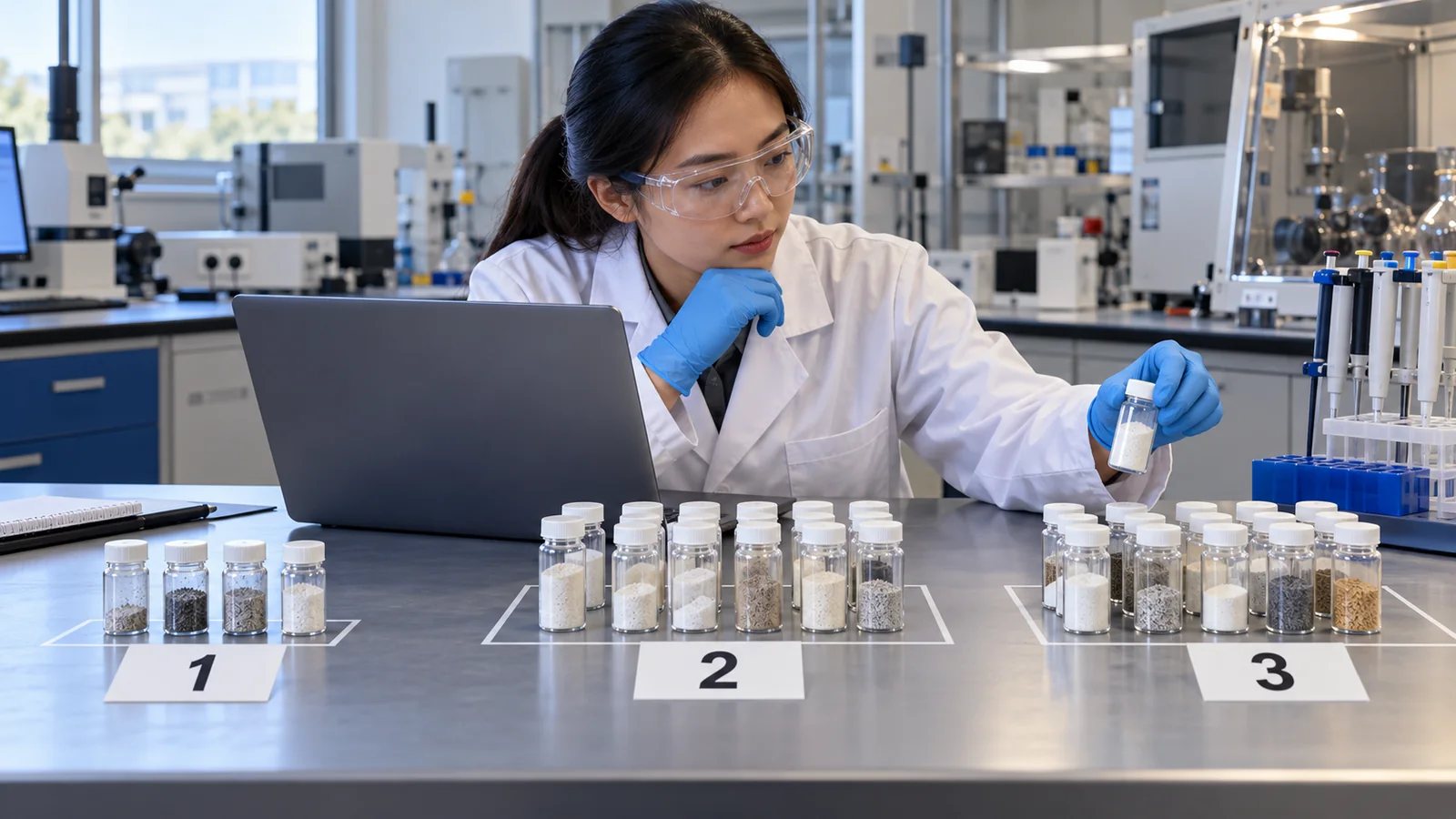
Experiments cost time, material and effort. You cannot try every combination of conditions (temperature, time, composition, concentration and so on). So there is a way to use the results so far to choose "the next measurement that looks most worthwhile": Bayesian optimization and active learning. This article explains the Gaussian process (a "best-guess line" and a "band of not knowing") and the acquisition function (the balance between exploring and exploiting) with figures and small calculations, and sorts out how these methods relate to design of experiments. It then looks at how much they help (a simple simulation of our own, and studies using experimental data) and the pitfalls in practice (noise, dimensions, constraints), from a materials engineer's viewpoint.
- The short version, what to know first, and where this fits in the series
- Finding the best conditions with few experiments: three approaches
- The Gaussian process: a "best-guess line" and a "band of not knowing"
- Where to measure next: acquisition functions, exploring and exploiting
- How it proceeds, step by step
- How much does it help?
- Active learning: improving the overall prediction, not finding the maximum
- The relationship with design of experiments (DoE)
- Pitfalls in practice
- Cases with experiments
- A materials engineer's view
- Limits, what we could not confirm, and a summary
- How to read the yardsticks and standards
- Glossary
- References
- Claim-to-source audit
Sourced = stated in a published source (linked)
Our calculation = a value computed in this article from the stated assumptions
Not yet confirmed = plans, targets, drafts, work in progress, outlooks: not settled
Our own reading for materials engineers is marked as commentary. Inference is shown in bold. Claims by research groups are labelled as claims.
1. The short version, what to know first, and where this fits in the series
- Bayesian optimization uses the results so far to choose the next experiment (or the next few) when every experiment is expensive. It has two parts: a guess about the response (a Gaussian process) and a rule for choosing what comes next (an acquisition function). The problems it is meant for typically allow at most a few hundred evaluations and about 20 or fewer input dimensions Sourced[Ref. 1]
- Bayesian optimization looks for the maximum; active learning improves the prediction overall. Both choose "the next point to measure" by using uncertainty. In a simple one-dimensional example of our own (our calculation), the share of runs that reached 98% or more of the true maximum after 10 experiments was 98% for Bayesian optimization and 29% for random choice Our calculation. But this is a made-up example, not a measure of real performance.
- In studies with experimental data, the benefit depends on conditions. There are cases where research is sped up by up to about 20 times compared with random choice, and cases where a poor choice of method makes it slower than random Sourced[Ref. 2]. The approach does not compete with design of experiments (DoE); the two can be combined.
"Bayesian" refers to the idea of "updating an initial guess after seeing data", much as a weather forecast is revised with each new observation. This article is about "using that updating to choose the next condition to test". In the series' common analogy, materials search is "looking for treasure on a vast map", and Bayesian optimization is a tool for deciding where to dig without digging everywhere. Machine learning is "an approximator that learns trends from past data" (see our explainer on machine learning and neural networks).
It helps to read our explainers on small-data machine learning (predicting with little data) and on uncertainty and applicability domain (how far to trust a prediction), and then this article (choosing the next experiment). Our explainers on closed-loop optimization and self-driving laboratories combine the methods here with hardware that runs the experiments.
2. Finding the best conditions with few experiments: three approaches
Suppose you want to fix the temperature, the time and the raw-material ratio for firing a material. With 10 values for each, that is 1,000 combinations. If one experiment takes a day, it takes about three years. How can you do fewer experiments?
| Approach | How points are chosen | Strengths | Weaknesses |
|---|---|---|---|
| Grid | Conditions are laid out at equal steps and all are measured | Simple; gives a view of the whole range | The number explodes as conditions are added |
| Random | Conditions are chosen at random | Simple; little bias | Does not use earlier results |
| Design of experiments (DoE) | A table of conditions is prepared in advance by statistical design, to study effects with few runs | Effects and interactions of factors can be read in an organised way | The number of runs and conditions are fixed at the start; it does not adapt to results |
| Bayesian optimization | The next condition is chosen from the results so far, then chosen again after each result | Approaches the maximum with few runs | Depends on model settings, noise and dimensions |
The arrangement of the table is Our calculation (organisation). Commentary based on the explanation of DOE in the NIST/SEMATECH e-Handbook [Ref. 3].
How fast does a grid grow as conditions are added? A full set of two levels (high and low) takes 2ᵏ runs for k factors, and a full set of three levels takes 3ᵏ runs. The NIST e-Handbook explains that a three-level full factorial design takes 9 runs for 2 factors and 27 runs for 3 factors Sourced[Ref. 3]. Extending the count gives the table below.
| Number of factors k | 2 | 3 | 4 | 5 | 6 |
|---|---|---|---|---|---|
| Full two-level design (2ᵏ runs) | 4 | 8 | 16 | 32 | 64 |
| Full three-level design (3ᵏ runs) | 9 | 27 | 81 | 243 | 729 |
The numbers in the table are Our calculation (powers; each added factor doubles or triples the count).
3. The Gaussian process: a "best-guess line" and a "band of not knowing"
The first part of Bayesian optimization is the Gaussian process. The name sounds hard, but what it does is this: "from the results at the points measured, it predicts the result at conditions not yet measured, together with a margin".
- The best-guess line (mean): it passes through the results measured and joins the points smoothly.
- The band of not knowing (uncertainty): narrow where there is data, wide far from the data.
- The assumption: "if conditions are close, the results should be similar". How close counts as similar is set by the kernel (its length scale).
In Frazier's tutorial, the Gaussian process starts from a "prior guess" about the function (a mean and a kernel), adds the data, and updates the guess. The prediction for an unmeasured condition is a normal distribution, and if measurements have no noise, the mean passes through the measured points and the uncertainty there is zero Sourced[Ref. 1]. The left panel of the figure shows this case. For a review of Bayesian optimization as a whole, see Shahriari et al. Sourced[Ref. 4].
With little data, there are countless lines that could pass through the points. The Gaussian process does not pick one; it shows the range of possible lines as a band. A wide band says "nobody has measured here yet, so we do not know". Using this "not knowing" to decide the next point is the heart of the method (next section).
Real measurements scatter (the same condition gives slightly different results). As in the right panel, if noise is taken into account, the band does not shrink to zero even at the measured points, because "this single measurement may be a little off the true value". Criteria such as EI may need adjustment when there is noise Sourced[Ref. 1].
In more detail: why you can think of it as a "weighted average that favours nearby points"
The mean of a Gaussian-process prediction can be written as a weighted sum of the measured results. The weights are set by the "closeness" (the kernel) between the condition to predict and each measured point, and closer points count more. The guess line is therefore a smooth line that leans heavily on nearby results. In our example the kernel's length scale was fixed at 0.1 (with conditions scaled to 0-1). In practice it can also be estimated from data (our setting).
4. Where to measure next: acquisition functions, exploring and exploiting
The second part is the acquisition function, a formula that gives each candidate condition a score. The condition with the highest score is measured next. The difficulty is that two urges pull against each other.
- Exploitation: measure where the current guess says the result will be good.
- Exploration: measure where we do not yet know. A better spot may be hiding there.
In fishing terms, dropping a line at your usual spot is exploitation, and trying a new spot is exploration. The acquisition function balances the two in a single number. Two common ones follow.
- Expected improvement (EI): the expected amount by which the next measurement would beat the best result so far. It was proposed by Močkus and became widely known through the EGO (efficient global optimization) algorithm of Jones et al. It scores highly the places where the guess is high and the uncertainty is also large Sourced[Refs. 5, 1].
- Upper confidence bound (UCB): "guess (mean) + κ × not knowing (standard deviation)". A larger κ leans toward exploration. Srinivas et al. gave this method a theoretical guarantee Sourced[Ref. 6].
Checking with a small numerical example
Suppose the best result so far is 0.90. There are three candidates, with the following guess (μ) and uncertainty (σ). Which should be measured?
| Candidate | Guess μ | Uncertainty σ | Probability of improvement (PI) | Expected improvement (EI) | UCB (κ=2) |
|---|---|---|---|---|---|
| A: the highest guess | 1.00 | 0.10 | 0.84 | 0.108 | 1.20 |
| B: a low guess, but very uncertain | 0.80 | 0.50 | 0.42 | 0.153 | 1.80 |
| C: in between | 0.95 | 0.30 | 0.57 | 0.146 | 1.55 |
The numbers in the table are Our calculation (a made-up example). EI = (μ − best) × Φ(z) + σ × φ(z), with z = (μ − best) / σ, where Φ is the cumulative distribution of the standard normal and φ its density. PI = Φ(z).
Choosing by probability of improvement (PI) alone picks A, because A has the highest chance of beating the best. But both EI and UCB pick B: although its mean is low, its uncertainty is large and it has a chance of a big win. A different acquisition function can mean a different choice. As the note beside the figure says, even with the same data, EI and UCB can peak at different places.
In more detail: what the EI formula means
The first term of EI, (μ − best) × Φ(z), stands for "exploitation" (large when the mean is well above the best). The second term, σ × φ(z), stands for "exploration" (large when the uncertainty σ is large). EI is zero at points already measured (when there is no noise) Sourced[Ref. 1].
5. How it proceeds, step by step
Bayesian optimization repeats: build the model, choose the next condition, run the experiment, add the data. With each experiment the band narrows and the next point changes.
In the example, after the third experiment there is little data and the band is wide, so we do not yet know much. After the fifth, experiments have gone near a high region, while regions not yet measured also remain candidates. After the eighth, experiments have been placed at both the first peak found and a different peak. Rather than staying with a local good spot, going to check another peak is the benefit of exploration.
6. How much does it help?
"How many fewer experiments will Bayesian optimization really need?" is what a materials engineer most wants to know. Let us look at it in two ways.
(1) A simple simulation of our own (one dimension, no noise)
- We used a made-up one-dimensional response with two peaks (maximum 0.90), made the first three experiments random, and chose the rest by EI. The numbers are averages over 200 runs Our calculation.
- After 10 experiments, the share of runs reaching 98% or more of the true maximum was 98% for Bayesian optimization and 29% for random choice. After 15 it was 100% and 40% Our calculation.
- The mean best value at 10 experiments was about 0.89 for Bayesian optimization and about 0.80 for random choice Our calculation.
The result above is for one dimension, no noise, and a kernel setting that suits the response, a favourable example. The authors of Olympus point out that optimization algorithms are typically tested on low-dimensional synthetic functions, so it is unclear how they would perform on noisy, higher-dimensional experimental tasks Sourced[Ref. 7]. Read it together with the studies on experimental data in (2) below.
(2) Studies using experimental data
- Rohr et al. (2020): on electrochemical catalyst data (four chemical spaces of 2,121 catalysts each, the overpotential for the oxygen evolution reaction) they compared sequential learning (choosing the next point with a model) with random choice. They report that research "can be accelerated by up to a factor of 20" in specific scenarios, while "certain choices of models are ill-suited" and cause substantial deceleration compared with random acquisition Sourced[Ref. 2].
- Liang et al. (2021): on five experimental materials systems they compared Gaussian processes, random forests and others. They report that a Gaussian process with anisotropic kernels and a random forest performed comparably and both outperformed a Gaussian process with isotropic kernels, with the anisotropic-kernel Gaussian process the most robust Sourced[Ref. 8].
Here "acceleration" means: given a data set in which every result has already been measured, let the method choose, and measure how many times faster than random choice it finds good points. In a real search the answers are unknown, and there may be good points outside the data set.
7. Active learning: improving the overall prediction, not finding the maximum
Bayesian optimization aimed at "finding the maximum". Sometimes the aim is different, for example "to grasp the whole relationship between composition and property with few experiments". Then you use active learning.
Settles' literature survey gives the core idea of active learning as: a learning algorithm can reach higher accuracy with fewer labelled training examples if it is allowed to choose the data it learns from. For materials, a "label" is a measured result. A typical way to choose is uncertainty sampling (measure the point where the prediction is least confident) Sourced[Ref. 9]. Lookman et al. describe active learning in materials science as a combination of "a surrogate model that provides uncertainties" and "a utility function that prioritises the next points" Sourced[Ref. 10].
- In our example, the same made-up response was predicted from 15 experiments. The overall prediction error (RMSE) was 0.024 when measuring where the model knows least and 0.113 for random choice (mean of 200 runs) Our calculation.
- Measuring where we know least spreads the conditions over the whole range. Random choice can bunch up (right-hand side of the figure).
- Bayesian optimization concentrates on "the top of the hill"; active learning spreads out over "the whole range". Different aims lead to different choices.
The table below sets the two side by side. In practice there are in-between cases (examine the neighbourhood of the maximum closely while also learning the whole picture). Lookman et al. also describe extensions to several properties and to data of differing fidelity (experiment and calculation) Sourced[Ref. 10].
| Item | Bayesian optimization | Active learning |
|---|---|---|
| Aim | Find the condition that maximises (or minimises) a target value such as yield or strength | Improve the prediction model over the whole range |
| Next point | Where improvement is expected (a balance of exploring and exploiting) | Where the prediction is least confident (and similar rules) |
| How success is measured | Best value so far; the number of runs until it is found | How far the prediction error falls with the number of experiments |
| Suited to | Searching for optimum conditions | Grasping trends and relationships overall, or reusing the model later |
The arrangement of the table is Our calculation (organisation). Commentary based on Settles [Ref. 9], Lookman et al. [Ref. 10] and Frazier [Ref. 1].
8. The relationship with design of experiments (DoE)
Design of experiments is a method with a long statistical tradition, widely used in materials and process work. The NIST e-Handbook describes design of experiments (DOE) as an efficient statistical procedure for planning experiments Sourced[Ref. 3]. How does it differ from Bayesian optimization, and how can they be combined?
| Item | Design of experiments (DoE) | Bayesian optimization |
|---|---|---|
| How conditions are decided | All conditions are decided first (in one batch) | The next is decided after seeing results (sequentially) |
| Good at | Reading the effects and interactions of factors; finding an optimum with a quadratic response surface (central composite and Box-Behnken designs and so on) | Getting close to the maximum with few runs; copes more easily with nonlinear, complicated responses |
| Ease of interpretation | High (effect sizes can be given as numbers) | Low (the model is a black box); interpretation methods can be applied afterwards |
| Assumptions | Many designs assume a response linear (or quadratic) in the parameters, with normally distributed errors of constant variance | Assumes a degree of smoothness in the response (the kernel) |
| Combining | Use it for the first few runs to grasp the overall picture | Then follow up while watching the results |
The arrangement of the table is Our calculation (organisation). Based on the NIST e-Handbook [Ref. 3] (it describes the central composite and Box-Behnken designs as classical designs for quadratic models introduced in the 1950s, and says quadratic models are almost always sufficient for industrial applications) and on ISO 3534-3:2013 [Ref. 11] (terms for designs in which the response is one-dimensional and continuous, its expectation is linear in the parameters, and the error is normal with constant variance).
In practice a natural flow is: (1) use DoE first to grasp how the factors act overall (which factors matter, whether there are interactions); (2) once candidates are narrowed, use Bayesian optimization to approach the optimum with few runs (commentary). The DoE results also become the first data for Bayesian optimization. When you need to explain "why this condition is good", the DoE response surface, or methods for interpreting results (see our explainer on explainable AI and materials insight), are useful.
9. Pitfalls in practice
Bayesian optimization is handy, but it does not "work automatically once you put it in". Here are the points a materials engineer should check first.
- Noise (reproducibility): if results at the same condition scatter, you cannot tell whether "good" was due to the condition or chance. Repeat measurements at the same condition to learn the scatter, and treat it as noise Sourced[Ref. 1]. Lot-to-lot and operator differences are part of the noise.
- Dimensions (number of conditions): Frazier says successful applications are typically of about 20 dimensions or fewer, and lists methods that work well in high dimensions as an open problem Sourced[Ref. 1]. With many conditions, it is realistic to narrow to the influential factors with DoE before using it (inference).
- Constraints: safety, cost and conditions you cannot synthesise (for example a dangerous temperature) must be excluded from the search. Extensions that handle constraints are known Sourced[Ref. 1].
- Parallel experiments: when you fire several samples at once in a furnace, you decide "the next few" rather than "the next one". Parallel EI and the Constant Liar heuristic are described Sourced[Ref. 1].
- Defining the goal: if cost or another property matters as well as yield, you must decide "what to maximise". Extensions to several properties are being studied Sourced[Ref. 10].
- Choice of model: Liang et al. showed that the choice of kernel for the Gaussian process changes the result Sourced[Ref. 8]. A default setting is not always the best.
The "not knowing" in this article is "we do not know because we have not measured yet" (model uncertainty). The scatter of measurements (the result changes even at the same condition) is a different concept, handled in the model as a separate noise term. If the two get mixed up, you cannot tell "a region not yet measured" from "a region where measurements merely scatter". Measuring the same condition a few times first to learn the scatter lets you tell them apart (commentary).
10. Cases with experiments
Here are some studies that connected Bayesian optimization or similar methods to experiments. All are reports (claims) by the research groups, under different conditions.
| Study | Target | What was reported | Reading note |
|---|---|---|---|
| Xue et al. (2016) | NiTi-based shape-memory alloys (aiming at a small thermal hysteresis ΔT) | From about 800,000 candidate compositions, 36 predicted compositions were synthesised and tested over 9 feedback loops. 14 had a smaller ΔT than any of the 22 in the original data; the smallest was 1.84 K for Ti50.0Ni46.7Cu0.8Fe2.3Pd0.2 Sourced[Ref. 12] | A study confirmed by experiment (synthesis and testing). We did not confirm a control against random selection |
| Shields et al. (2021) | Reaction conditions in organic synthesis (Pd-catalysed direct arylation and others) | Compared the decisions of human experts with Bayesian optimization through an online game, and report that Bayesian optimization is better in average efficiency (number of experiments) and consistency. Also applied to two other reactions Sourced[Ref. 13] | A comparison on specific reactions, with conditions on the human side such as the information shown when choosing |
| Rohr et al. (2020) | Experimental data on oxygen-evolution catalysts (four spaces, 2,121 each) | Up to about 20 times acceleration over random choice; for some choices, slower than random Sourced[Ref. 2] | A comparison on data sets in which everything was already measured (retrospective) |
| Liang et al. (2021) | Five experimental materials systems | The Gaussian process with anisotropic kernels and the random forest were comparable and better than the isotropic kernel Sourced[Ref. 8] | A comparison of models. Results on five systems do not guarantee the same for every system |
Each number is a value under the conditions of its own paper. The arrangement of the table is Our calculation (organisation). Checked on 22 October 2026.
Japanese research groups have also adapted Bayesian optimization to materials science. For example, COMBO (Ueno et al., 2016) is a Bayesian optimization library for materials science Sourced[Ref. 14]. The review by Terayama et al. frames the search in chemistry and materials as "black-box optimization", and describes combining methods such as Bayesian optimization, reinforcement learning and active learning with simulations based on quantum mechanics or molecular mechanics, and with experiments Sourced[Ref. 15].
11. A materials engineer's view
Bayesian optimization works by gradually adding pairs of conditions (inputs) and results (outputs). For that, in day-to-day lab notebooks: (1) write conditions as numbers ("2 h 15 min", not "a bit longer"); (2) measure results with the same metric, under the same conditions; (3) record failed experiments too (a poor result is important information for the model); (4) note the lot, the equipment and the operator (sources of noise). The FAIR principles (data that are findable, accessible, interoperable and reusable) are one way of thinking about keeping data in a form that machines can use Sourced[Ref. 16].
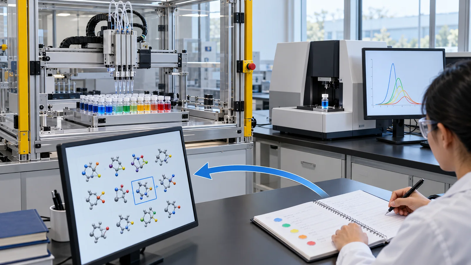
AI (the acquisition function) is good at showing numerically "where measuring pays off". Experts decide: (1) the search range (excluding physically impossible conditions); (2) constraints (safety, cost, equipment limits); (3) what counts as good (yield alone, or cost as well); (4) checking the results (is an outlier a measurement error or a genuinely good condition? re-measure at the same condition). Rather than running the AI's proposal as it stands, an expert checks it before measuring, which is both safer and more efficient (commentary).
For the optimum found, check: (1) does it reproduce over several runs under the same condition (learn the range of scatter); (2) is it the same with another lot or another piece of equipment; (3) does the result hold up around the optimum (conditions shifted a little), which is robustness; (4) is it really better than the current condition (the control), measured the same way. A method that searches for a maximum tends to pick a point where a high value appeared by chance. Always include a confirmation experiment (commentary).
12. Limits, what we could not confirm, and a summary
(1) What we could not confirm
- From the abstract we could not confirm whether the study by Xue et al. (2016) included a control experiment against random or conventional methods.
- We did not confirm the detailed conditions of the comparison between humans and Bayesian optimization in Shields et al. (2021), such as the number of participants; we stay within the abstract.
- For the "about 20 times" of Rohr et al. (2020) we stay within the abstract and do not give the specific setting that produced it.
- Our simulation is a made-up one-dimensional, noise-free case; we did not compute results for many dimensions or with noise.
- We could not confirm an international standard specific to Bayesian optimization or active learning.
- Bayesian optimization chooses the next condition with a Gaussian process (a guess line and a band of not knowing) and an acquisition function (a score for the next point). It balances exploration (where we do not know) and exploitation (where it looks good) in a single number Sourced
- A different acquisition function can pick a different point. In the made-up example, PI picked the point with the highest guess, and EI and UCB picked the most uncertain point Our calculation
- Active learning measures where we do not know, to improve the "overall prediction". In our example, after 15 experiments the overall error was about one fifth of that of random choice Our calculation
- The benefit depends on conditions. Both cases of up to about 20 times faster than random choice and slower cases are reported. Check both the results on experimental data and your own system Sourced
- It can be combined with design of experiments. Watch noise, dimensions (about 20 or fewer), constraints and parallel experiments, and always confirm the optimum with repeat experiments Sourced
13. How to read the yardsticks and standards
The first yardstick of Bayesian optimization and active learning is the best value found per number of experiments (optimization), or the prediction error per number of experiments (active learning). Next come what it was compared with (random, humans, other methods) and on what data it was tried (real experiments, or a data set already measured in full). Checked on 22 October 2026.
| Item | Representative benchmarks and methods (name, source) | Standards and guidance (ISO/IEC, NIST, etc.) | Reading notes |
|---|---|---|---|
| Performance of optimization (acceleration) | Rohr et al.: quantifies acceleration (up to about 20 times) and deceleration relative to random [Ref. 2]Sourced Liang et al.: defines acceleration and enhancement metrics across five experimental materials systems [Ref. 8]Sourced | Not found (we did not find an international standard defining how to evaluate Bayesian optimization) | Comparisons on data sets whose answers are known. A real search is unknown |
| Optimization of noisy experiments | Olympus: a framework for comparing optimization methods on data that emulate experiments (Häse et al. 2021) [Ref. 7]Sourced | Not found | Performance on synthetic functions does not carry over directly to noisy, high-dimensional experiments |
| Performance of active learning | Learning curves (prediction error against number of experiments). Settles' survey and the review of Lookman et al. on materials science [Refs. 9, 10]Sourced | Not found | Compare with random selection at the same number of experiments |
| Terms and designs of experiments | NIST/SEMATECH e-Handbook, "5. Process Improvement" (design of experiments, response surface methods) [Ref. 3]Sourced | ISO 3534-3:2013, Statistics - Vocabulary and symbols - Part 3: Design of experiments (published April 2013; confirmed again in 2024) [Ref. 11]Sourced | A vocabulary standard; it does not prescribe a Bayesian optimization procedure. The text is paid and we did not check its requirements |
| Handling of data | FAIR principles (Wilkinson et al. 2016) [Ref. 16]Sourced | Recommended principles (no legal force) | Guidance for keeping experimental data in machine-usable form |
The arrangement of the table is Our calculation (organisation). Numbers, titles and status were checked on the ISO page (22 October 2026). The text of the standard is paid, so we limit ourselves to its title and scope and do not state requirements.
Reading notes (for materials engineers)
- An "acceleration" figure is a value on a data set whose answers are known: in a real search the answers are unknown. Use the numbers as a rough guide when choosing a method [Refs. 2, 8]
- A search for the maximum tends to pick values that are high by chance: confirm the best point found with repeat experiments (commentary)
- Standards are recommendations or vocabulary: ISO 3534-3 is a vocabulary standard and does not guarantee a search procedure. Standards generally gain binding force only when cited in laws or contracts (commentary) [Ref. 11]
14. Glossary
- Bayesian optimization
- A method that uses results so far to choose the next condition, approaching the maximum (or minimum) with few runs.
- Active learning
- Learning in which the next point is chosen so as to improve the prediction model.
- Gaussian process
- A method that predicts the result at unmeasured conditions from the measured points as a mean (guess) and a margin (uncertainty).
- Kernel / length scale
- A function that says "close conditions give similar results" / a measure of how far apart conditions must be before they stop resembling each other.
- Acquisition function
- A formula that scores candidate conditions. The condition with the top score is measured next.
- Exploration and exploitation
- Exploitation = measure where it looks good. Exploration = measure where we do not know.
- Expected improvement (EI)
- The expected amount by which the next run would beat the best so far.
- Probability of improvement (PI)
- The probability that the next run beats the best so far.
- Upper confidence bound (UCB)
- Mean of the guess + κ × standard deviation. A larger κ means more exploration.
- Uncertainty sampling
- An active-learning rule that measures next the point where the prediction is least confident.
- Black-box function
- A function with no known formula: you put values in and look at the result, such as the response of an experiment.
- Design of experiments (DoE)
- A statistical method for planning experiments efficiently with few runs.
- Response surface methodology
- A method that approximates the relation between conditions and results with a surface (often quadratic) to find an optimum.
- Factor / level
- A condition that is varied (such as temperature) / its values (such as high and low).
- Noise
- Scatter in measurements: the result changes a little even at the same condition.
- Dimensions
- The number of conditions (factors).
- Constraint
- A range of conditions that must not be searched (safety, cost, equipment limits and so on).
- Batch (parallel) experiments
- Deciding the next several conditions at once and running them together.
- RMSE
- The square root of the mean squared difference between prediction and answer. A guide to overall prediction error.
- Retrospective evaluation
- Evaluating a method on a data set in which everything has already been measured.
- FAIR principles
- Guidance for making data findable, accessible, interoperable and reusable.
15. References
- Frazier P. I. "A tutorial on Bayesian optimization", arXiv:1807.02811 (2018) — arxiv.org/abs/1807.02811
- Rohr B. et al. "Benchmarking the acceleration of materials discovery by sequential learning", Chem. Sci. 11, 2696–2706 (2020), DOI 10.1039/C9SC05999G — doi.org/10.1039/C9SC05999G
- NIST/SEMATECH "e-Handbook of Statistical Methods, Chapter 5 "Process Improvement" (design of experiments, response surface designs)", (NIST Information Technology Laboratory) — itl.nist.gov/div898/handbook/pri/pri.htm
- Shahriari B. et al. "Taking the human out of the loop: a review of Bayesian optimization", Proc. IEEE 104, 148–175 (2016), DOI 10.1109/JPROC.2015.2494218 — doi.org/10.1109/JPROC.2015.2494218
- Jones D. R., Schonlau M., Welch W. J. "Efficient global optimization of expensive black-box functions", J. Global Optim. 13, 455–492 (1998), DOI 10.1023/A:1008306431147 — doi.org/10.1023/A:1008306431147
- Srinivas N. et al. "Gaussian process optimization in the bandit setting: no regret and experimental design", ICML 2010, arXiv:0912.3995 — arxiv.org/abs/0912.3995
- Häse F. et al. "Olympus: a benchmarking framework for noisy optimization and experiment planning", Mach. Learn.: Sci. Technol. 2, 035021 (2021), DOI 10.1088/2632-2153/abedc8 — doi.org/10.1088/2632-2153/abedc8
- Liang Q. et al. "Benchmarking the performance of Bayesian optimization across multiple experimental materials science domains", npj Comput. Mater. 7, 188 (2021), DOI 10.1038/s41524-021-00656-9 — doi.org/10.1038/s41524-021-00656-9
- Settles B. "Active learning literature survey", Computer Sciences Technical Report 1648, University of Wisconsin-Madison (2009) — minds.wisconsin.edu/handle/1793/60660
- Lookman T. et al. "Active learning in materials science with emphasis on adaptive sampling using uncertainties for targeted design", npj Comput. Mater. 5, 21 (2019), DOI 10.1038/s41524-019-0153-8 — doi.org/10.1038/s41524-019-0153-8
- ISO "ISO 3534-3:2013 Statistics — Vocabulary and symbols — Part 3: Design of experiments", (ISO page) — iso.org/standard/44245.html
- Xue D. et al. "Accelerated search for materials with targeted properties by adaptive design", Nat. Commun. 7, 11241 (2016), DOI 10.1038/ncomms11241 — doi.org/10.1038/ncomms11241
- Shields B. J. et al. "Bayesian reaction optimization as a tool for chemical synthesis", Nature 590, 89–96 (2021), DOI 10.1038/s41586-021-03213-y — doi.org/10.1038/s41586-021-03213-y
- Ueno T. et al. "COMBO: an efficient Bayesian optimization library for materials science", Mater. Discov. 4, 18–21 (2016), DOI 10.1016/j.md.2016.04.001 — doi.org/10.1016/j.md.2016.04.001
- Terayama K., Sumita M., Tamura R., Tsuda K. "Black-box optimization for automated discovery", Acc. Chem. Res. 54, 1334–1346 (2021), DOI 10.1021/acs.accounts.0c00713 — doi.org/10.1021/acs.accounts.0c00713
- Wilkinson M. D. et al. "The FAIR guiding principles for scientific data management and stewardship", Sci. Data 3, 160018 (2016), DOI 10.1038/sdata.2016.18 — doi.org/10.1038/sdata.2016.18
16. Claim-to-source audit
| Claim in the text | Basis | Category |
|---|---|---|
| What Bayesian optimization targets (costly derivative-free black boxes, up to a few hundred evaluations, usually 20 or fewer dimensions); the Gaussian process (mean and kernel; with noiseless data the mean passes through the data and the uncertainty is zero there); the definition of EI and its preference for uncertain regions; EI being zero at measured points; proposal by Močkus and popularisation by Jones et al.; EI needing adjustment under noise; constraints, parallel evaluation (Constant Liar) and multi-fidelity; high dimensions as an open problem; use of Bayesian optimization to choose experiments in materials and drug design | Reference 1 https://arxiv.org/abs/1807.02811 | Sourced |
| The review of Bayesian optimization (Shahriari et al.); EGO (Jones et al. 1998); GP-UCB and regret bounds based on information gain (Srinivas et al.) | Reference 4 https://doi.org/10.1109/JPROC.2015.2494218 Reference 5 https://doi.org/10.1023/A:1008306431147 Reference 6 https://arxiv.org/abs/0912.3995 | Sourced |
| The core idea of active learning (a learner that chooses its data can reach higher accuracy with fewer labelled examples), uncertainty sampling, the three scenarios (membership query synthesis, stream-based, pool-based); active learning in materials science (uncertainty plus a utility function; extension to multiple properties and multi-fidelity data) | Reference 9 https://minds.wisconsin.edu/handle/1793/60660 Reference 10 https://doi.org/10.1038/s41524-019-0153-8 | Sourced |
| Xue et al.: NiTi-based shape-memory alloys, about 800,000 candidate compositions, 36 compositions synthesised and tested over 9 feedback loops, 14 with a smaller ΔT than any of the original 22, smallest 1.84 K (Ti50.0Ni46.7Cu0.8Fe2.3Pd0.2) | Reference 12 https://doi.org/10.1038/ncomms11241 | Sourced |
| Shields et al.: a benchmark for Pd-catalysed direct arylation, comparison with expert chemists through an online game, Bayesian optimization better in average efficiency and consistency (the authors' claim), application to Mitsunobu and deoxyfluorination reactions | Reference 13 https://doi.org/10.1038/s41586-021-03213-y | Sourced |
| Rohr et al.: four chemical spaces of 2,121 catalysts each, oxygen-evolution overpotential, up to a factor of 20 acceleration over random, and substantial slowdown for some choices. Liang et al.: five experimental materials systems; GP with anisotropic kernels and random forests comparable and better than isotropic GP, anisotropic GP the most robust. Olympus: a framework for benchmarks emulating experiments, noting that evaluation has leaned on low-dimensional synthetic functions | Reference 2 https://doi.org/10.1039/C9SC05999G Reference 8 https://doi.org/10.1038/s41524-021-00656-9 Reference 7 https://doi.org/10.1088/2632-2153/abedc8 | Sourced |
| COMBO (a Bayesian optimization library for materials science); the black-box optimization framing (Bayesian optimization, reinforcement learning, active learning; combination with simulation and experiments) | Reference 14 https://doi.org/10.1016/j.md.2016.04.001 Reference 15 https://doi.org/10.1021/acs.accounts.0c00713 | Sourced |
| NIST e-Handbook: the place of DOE; a three-level full factorial needs 9 runs for 2 factors and 27 for 3; response surface designs (central composite and Box-Behnken designs are classical designs for quadratic models introduced in the 1950s; quadratic models almost always suffice in industry). ISO 3534-3:2013: number, title, April 2013 publication, reconfirmed in 2024, scope. The FAIR principles | Reference 3 https://www.itl.nist.gov/div898/handbook/pri/pri.htm Reference 11 https://www.iso.org/standard/44245.html Reference 16 https://doi.org/10.1038/sdata.2016.18 | Sourced |
| The one-dimensional response in the figures (two peaks, maximum 0.90), the Gaussian-process curves (kernel length scale 0.1), the EI and UCB curves, the acquisition-function example (PI, EI, UCB), the share of runs reaching 98% or more of the maximum at 10 experiments (Bayesian optimization 98%, random 29%) and at 15 (100%, 40%), mean best values (at 10: 0.89 vs 0.80), the overall error of active learning (RMSE at 15: 0.024 vs 0.113), and the 2^k and 3^k run counts | our calculation (Python and NumPy; mean of 200 runs) | Our calculation |
| Whether Xue et al. had a control experiment, the detailed conditions of the Shields et al. comparison, the specific setting behind the "factor of 20" of Rohr et al., simulations in many dimensions with noise, and an international standard specific to Bayesian optimization or active learning | not confirmed in the primary sources we could access, so not stated (commentary) | commentary |
| The readings on how to divide DoE and Bayesian optimization, turning lab notes into data, the split of work between AI and experts, designing the confirmation of an optimum, and separating noise from model uncertainty | our own organisation and commentary based on the published content; not views stated by the research groups | commentary |
| Note on figure types: Figs 2, 3, 4, 5, 6, 7 include our calculation, Figs 8 are concept diagrams (vector drawings), and Figs 1, 9 are ImageGen-generated conceptual illustrations | a note by this article (commentary) | commentary |
Last updated: 22 October 2026. Sources are limited to primary material (peer-reviewed papers, arXiv papers, and official NIST and ISO pages). The simulations and numerical examples (the curves in the figures, the acquisition-function table, the run counts against the number of factors) are our own calculations, not results for real materials. We could not confirm whether Xue et al. had a control experiment, the detailed conditions of the Shields et al. comparison, the specific setting behind the "factor of 20" of Rohr et al., simulations in many dimensions with noise, or an international standard specific to Bayesian optimization or active learning, so we do not state them. All figures are concept diagrams or diagrams that include our own calculation; the ImageGen images are conceptual illustrations.