TECHNOLOGY EXPLAINER
Materials Data and Descriptors
— Turning a material into a “number card”, and facing data quality, missing values and bias
Machine learning can read only numbers. So the composition, structure and process of a material must first be turned into numbers. This list of numbers is a descriptor; in this series it is the material's “business card”. Which card you make, and the quality of the data you collect (scatter, missing values, bias, whether failures are recorded), strongly affects whether predictions come true. For materials engineers who want to put their own experimental data into a form MI can use, this article explains how descriptors are made and the pitfalls of data quality, with small calculations.
- Three-line summary, prerequisites, and where this fits in the series
- What a descriptor is: a material as a “business card” in numbers
- Making a card from composition: checking by hand
- Putting lab notes into a table: one row per sample, and data quality
- Putting numbers on the same scale
- Missing values and “could not be measured”
- Biased data, and the danger of extrapolation
- The value of failed results
- How to choose and reduce descriptors
- Limits, what we could not confirm, and a summary
- How to read the yardsticks and standards
- Glossary
- References (primary sources)
- Claim-to-source audit
Sourced = stated in a published source (reference link given)
Our calculation = a value this article computed from stated assumptions
Not yet confirmed = plans, revisions in progress and other matters not yet settled
Our reading of what this means for materials research is labeled commentary. An Inference is shown in bold.
The numbers in Chapters 5 to 7 are calculations on synthetic data that we generated (fixed random seed). They do not show real materials data or the performance of any product; they are examples to show mechanisms and pitfalls in numbers. The element values in Chapter 3 come from PubChem's periodic-table data, and the calculation is ours. For ISO/IEC and ISO standards we only checked the number, title and publication date, and have not read the full text.
1. Three-line summary, prerequisites, and where this fits in the series
- A descriptor is a “business card” of a material in numbers. It turns composition, structure and process into a list of values a machine can read. The choice of items on the card changes how well predictions come true
- Data quality decides prediction quality. Measurement scatter, differences in scale, missing values, bias in the data and whether failures are recorded all distort the result. Tidying the data is worth more than cleverness in the model
- The one point to remember: “could not be measured” and “did not work” are also data. If you keep them with a reason instead of leaving a blank, the “boundary” of where MI can be used becomes visible
You do not need to have read the introduction to materials informatics in this series; we explain the needed background briefly. The key points: machine learning is “an approximator that learns trends from past data,” and it is weak outside the range of the data (extrapolation). A descriptor is a “business card” of a material in numbers. Basic knowledge of chemistry and materials is enough; no programming is needed.
This is the second article in our series on materials informatics, after the introduction. The ideas of the “card” and of “data quality” built here are the base for the next articles: materials databases and the FAIR principles (how data are collected and shared), machine learning with small data (learning from little data), and uncertainty and applicability domain (how far a prediction can be trusted).
2. What a descriptor is: a material as a “business card” in numbers
(1) An analogy: comparing people you have just met, by their business cards
When you meet someone new, a business card helps you compare people. It has fixed items in a row: company, title, location. Materials work the same way. If there is a business card with fixed items written as numbers, a machine can calculate how similar two materials are. That card is a descriptor (also called a fingerprint). The review by Ramprasad and colleagues explains that predictions take the form “first express the material as numbers, then link that representation to the target property through a learned mapping,” and that these numerical representations can be of many types and scales depending on the applicationSourced [Ref. 1].
View original SVG, values and sources
Original SVG reference: Chart including our calculation (vector drawing). The idea of a "business card": a material turned into numbers from its composition, structure and process. Only the composition rows are actual calculations; the others show example items.
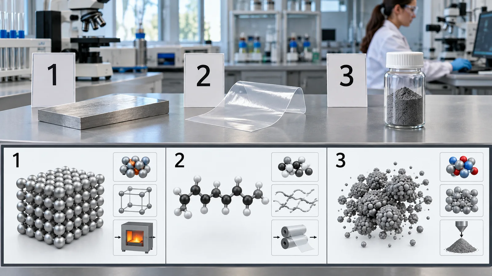
The items on a card fall roughly into three groups, according to where they come from: the composition (what is in it, and in what proportions), the structure (how the atoms are arranged), and the process (temperature, time, atmosphere and the like). As in Fig. 2, composition items can be calculated from the chemical formula alone. Structure and process items need other information.
| Type of card | How it is made / representative examples (source) | Strength | Caution |
|---|---|---|---|
| Composition descriptors | Statistics of element properties built from the formula (elements and proportions). The general-purpose framework of Ward et al. uses 145 attributes; its elemental-property statistics are the mean, mean absolute deviation, range, minimum, maximum and mode of 22 elemental properties [Ref. 3]Sourced. Matminer is software that gathers 47 featurization classes and can generate thousands of descriptors [Ref. 4]Sourced | No crystal structure needed. Built from the formula alone, so it can be computed at once for unknown compositions | The same composition can have different crystal structures with different properties; this card cannot tell them apart (commentary) |
| Structure descriptors | Built from atomic positions. Rupp et al. proposed a machine-learning model that predicts atomization energies of organic molecules from nuclear charges and atomic positions only [Ref. 5]Sourced. Bartók et al. reviewed descriptors of atomic environments (including SOAP) and state that they must be invariant to rotation, reflection, translation and exchange of like atoms [Ref. 6]Sourced | Reflects differences in how atoms are arranged | Needs a structure. For an unknown material the structure itself has to be predicted or computed, and that error mixes in (commentary) |
| Molecular fingerprints | Lists which substructures of a molecule are present. ECFP (extended-connectivity fingerprints) are circular fingerprints developed specifically for structure-activity modeling [Ref. 8]Sourced | Fast to compute, and easy to interpret as substructures | Does not directly express three-dimensional shape or the material's aggregate state (crystal, entangled polymer chains) (commentary) |
| Process descriptors | Turn how the material is made into numbers or categories: firing temperature, time, atmosphere, raw-material lot. Ling et al. report a framework for designing experiments that handles both composition and processing in optimization [Ref. 27]Sourced | Lets the model include the factors that actually govern performance | Quality depends on how well things are recorded. Conditions not measured (humidity, drying history) cannot be written on the card (commentary) |
The arrangement of this table is our own commentary. For other representations (spectra, images, text) and a detailed comparison of structure-based methods, see the reviews by Musil et al. [Ref. 9] and Damewood et al. [Ref. 10].
Books say “descriptor,” “feature,” “explanatory variable” or “attribute,” but here they all mean the same thing (commentary). Ghiringhelli and colleagues call the choice of descriptor a “largely silent, nonchallenged step” of statistical learning, and argue that when the scientific connection between the descriptor and the mechanisms behind the property is unclear, the causality of the learned relation is uncertainSourced [Ref. 2]. Do not choose card items casually; choose meaningful ones that match what you want to know.
3. Making a card from composition: checking by hand
Let us build the simplest card by hand. Our example material is LiFePO₄ (lithium iron phosphate). It contains lithium (Li), iron (Fe), phosphorus (P) and oxygen (O) in the ratio 1 : 1 : 1 : 4, seven atoms in all.
- Find the fractions. Li, Fe and P are 1/7 each, and O is 4/7
- Look up an element property. We use electronegativity (a rough measure of how strongly an atom pulls electrons). The PubChem periodic-table values are Li 0.98, Fe 1.83, P 2.19 and O 3.44 [Ref. 19]
- Take the fraction-weighted mean. (0.98 + 1.83 + 2.19) ÷ 7 + 4 × 3.44 ÷ 7 = 0.714 + 1.966 = 2.68
- Take the range. maximum − minimum = 3.44 − 0.98 = 2.46
The table at the bottom of Fig. 3 shows the “cards” made by the same steps for four compounds (Our calculation). The mean electronegativity is 2.68 for LiFePO₄, 2.55 for BaTiO₃, 2.05 for NaCl and 2.38 for MgO. The range (the difference between largest and smallest) can be read as larger for compounds with stronger ionic character (commentary). The “elemental property statistics” in the framework of Ward et al. extend this idea (mean, range and so on) to 22 element properties [Ref. 3].
Our calculation. Element values are from PubChem's periodic-table data [Ref. 19]. Means are weighted by atom fractions. This is a two-item introductory example; real composition descriptors have dozens to hundreds of items [Ref. 3].
Because the mean alone can be the same for NaCl (Na 0.93 and Cl 3.16) and for a compound of two elements with middling electronegativity. The range shows how different the elements are from each other. Think of it as one number covering what another number cannot show. Limit of the analogy: this card is made from the formula and says nothing about “how things are arranged.” Materials with the same composition and different structures get the same card.
4. Putting lab notes into a table: one row per sample, and data quality
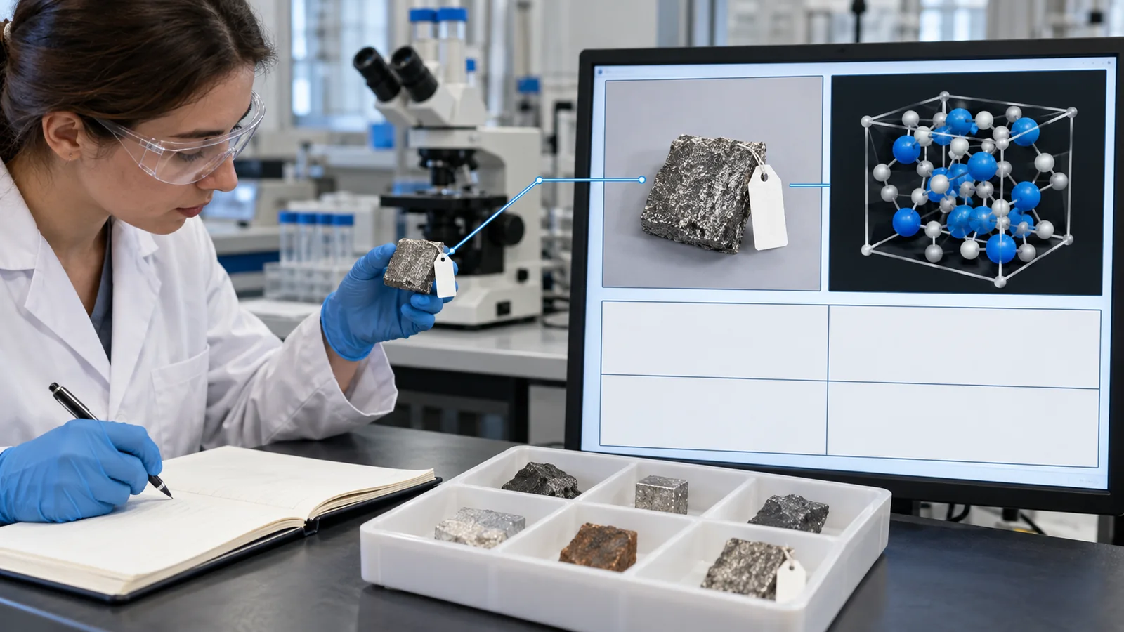
When you use your own experimental data, the first job is to put the laboratory notebook into a table. Machines read tables. Text and photos alone cannot be turned into numbers. Fig. 4 shows an example of turning free-text notes into a table with one row per sample.
View original SVG, values and sources
Original SVG reference: Conceptual diagram (vector drawing). An example of turning notes into a machine-readable table: conditions and results in separate columns, with units, lots and failures recorded. Values are for illustration.
There are only three rules for the table. (1) One row per sample (if you measure the same sample several times, add that many rows). (2) One column per item (put the unit in the column name). (3) Do not leave blanks (if something could not be measured or failed, write why). Just this makes later work much easier.
| Data-quality check | What happens | How to check (commentary) |
|---|---|---|
| Mixed units | °C and K, or MPa and GPa, end up in one column and the orders of magnitude do not match | Fix a unit for each column and write it in the column name. Check the range when importing |
| Spelling variants | “LiFePO4,” “LFP” and “lithium iron phosphate” are treated as different things | Standardize material names and abbreviations. Keep a separate formula column |
| Date, lot, instrument | You cannot tell which raw material, instrument or day a sample belongs to, so you cannot trace the cause of scatter | Always include columns for date, raw-material lot, instrument and operator |
| Detection limit, measurement range | “Below the measurement limit” gets recorded as a blank or as zero | Record the limit value, and the fact that the result was below it, in separate columns (Chapter 6) |
| Duplicates | The same sample enters twice and the evaluation becomes too lenient (a kind of data leakage) | Look for duplicates by sample ID. Treat repeats of one sample as one “group” |
| Outliers | You cannot tell whether it is an input error or a real phenomenon | Go back to the original record. Do not delete it while the reason is unknown |
| Measurement scatter | A model's error cannot go below the scatter of the measurement | Measure one sample repeatedly, and look at lot-to-lot and instrument-to-instrument differences (below) |
This table is our own commentary. The international standards on data quality (the ISO/IEC 5259 series) are introduced by title and scope in Chapter 11.
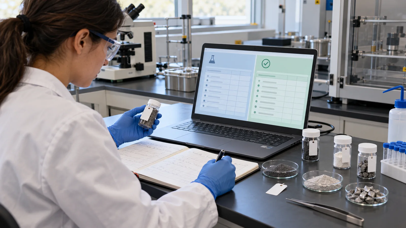
Here is one example of measurement scatter in numbers. The OQMD paper reports that the mean absolute error between experiments measuring the formation energy of the same compound is 0.082 eV/atom, “surprisingly large” (the DFT-versus-experiment difference is 0.096 eV/atom)Sourced [Ref. 16]. How to handle measurement scatter is organized in the field of metrology. For example, JCGM 100:2008 (the GUM) defines uncertainty of measurement as a parameter, associated with the result of a measurement, that characterizes the dispersion of the values that could reasonably be attributed to the measurandSourced [Ref. 26].
Make and measure the same sample three times, preferably from different lots. That scatter (a standard deviation, for example) is a rough floor for the error a model can aim for. If the scatter is 10%, a model claiming a 5% error is claiming an error smaller than the measurement itself, and it very likely memorizes noise (overfitting) (commentary).
Also, keep differences in lot (the production unit of a raw material) and instrument in the table as “differences in conditions,” not as “differences in the material.” Later you can then check “which lot was off.”
5. Putting numbers on the same scale
The items on a card often differ by orders of magnitude. Temperature, for example, runs from 300 to 1,300 K (a span of about 1,000), while a composition fraction runs from 0 to 1 (a span of 1). Many machine-learning methods are affected by such differences. The scikit-learn user guide explains that many estimators may behave badly if the individual features do not more or less look like standard normally distributed data (Gaussian with zero mean and unit variance)Sourced [Ref. 17].
We check the effect with a small experiment (Our calculation). We use a nearest-neighbor method, which “returns the mean value of the three closest past samples,” with two descriptors, temperature and fraction. The true property depends strongly (and periodically) on the fraction and only gently on temperature. We train on 60 points and measure the error on 500 new points (average of 30 runs).
The result is in Fig. 6. Without putting the numbers on one scale, distance is decided almost entirely by the difference in temperature, and the effect of the fraction is not seen. The error (RMSE) is 0.83, worse than the do-nothing prediction that just returns the mean (0.73). After standardization (subtracting each item's mean and dividing by its spread), the error falls to 0.24.
Our calculation. Synthetic data (true property = sin(2π × fraction) + 0.3 × (temperature − 800)/500 + noise 0.05). Not a result on real materials. For standardization, the mean and spread were computed from the training data only and applied to the test data (to avoid data leakage).
If the mean and spread used for standardizing are computed including the data used for evaluation, information from the evaluation leaks into training. Learn the standardization from the training data only, and just apply those values to the evaluation data (this is one of the “preprocessing” leaks organized by Kapoor and NarayananSourced [Ref. 22]; see our explainer on the basics of machine learning and neural networks). Some methods, such as those based on decision trees, are less sensitive to differences in scale, but we did not check primary sources on that here.
6. Missing values and “could not be measured”
Blanks (missing values) are common in materials tables: items not measured, samples that could not be measured, values outside the instrument's range. The scikit-learn user guide explains that a basic strategy for using incomplete datasets is to discard whole rows or columns containing missing values, but this comes at the price of losing data that may be valuable; a better strategy is to impute the missing values, that is, to infer them from the known part of the data [Ref. 18].
But why the values are missing matters. If values are not missing by chance, for example when “the lower the value, the more likely it falls below the detection limit and cannot be measured,” then collecting only the measured points creates a bias. We check this with a small experiment (Our calculation).
- Setup. Descriptor x (for example, the amount of an additive) and property y are related by y = x + noise (standard deviation 0.5). Values of y below −0.5 fall under the detection limit and are not recorded (about 33% of all values are missing)
- The true mean is 0.00. But the mean of the measured points alone rises to 0.60
- The slope is 1.00 for all points, but 0.82, gentler, for the measured points alone
- If we fill the missing values with the detection-limit value (−0.5), the mean is 0.24, still different from the true 0.00
Our calculation. Synthetic data (means and slopes computed from 200,000 points; the plot shows 200 points). Not a result on real materials.
Depending on why values are missing, it does not. Filling with the mean is a handy method that is often used when values are missing by chance, but when “lower values go missing,” you would be filling with the biased mean of the measured points alone, and the bias remains. In the example above, filling with the measured-only mean of 0.60 does not bring us closer to the true mean of 0.00. What to do: (1) record the reason for missing values (detection limit, failure, not measured) in a separate column; (2) treat “below the detection limit” as information in itself; (3) ask the person who measured about the reason (commentary).
7. Biased data, and the danger of extrapolation
If the data you collected are concentrated in part of the range of conditions, predictions will not come true outside that range. We check this with a small experiment (Our calculation). Let the true relation be y = sin(3x) + 0.5x, and train on 30 points (noise 0.05) measured only in x = 0 to 1. We evaluate inside that range and at x = 1 to 3 (outside).
The result is in Fig. 8. Inside the range, the error is 0.03 for the cubic polynomial and 0.08 for the 3-nearest-neighbor method; both are accurate. Outside (x = 1 to 3), the polynomial's error jumps to 12.6 (median). The 3-nearest method stays constant at the edge value, with an error of 0.98. That is about the same as the spread of the true values outside (standard deviation 0.97), no better than a “return the mean” prediction.
Our calculation. Synthetic data. Average of 50 runs (median for the polynomial). Outside the range, the way models fail depends on the model type (running away, or going flat), but neither is right.
This is an artificial and extreme example. But similar bias has been reported in real materials data. Jia and colleagues found, in reports of hydrothermal synthesis of amine-templated metal oxides, that the choice of amine follows a power-law distribution in which 17% of the amines occur in 79% of the reported compounds. Fashion and cognitive bias in how people choose experiments show up in the data. They further showed with 548 randomly generated experiments that the popularity of reactants and the choice of reaction conditions are uncorrelated with whether the reaction succeeds, and reported that models trained on a smaller randomized dataset outperformed models trained on larger human-selected datasetsSourced [Ref. 13].
Li and colleagues also showed, for several large materials datasets, that up to 95% of the data can be removed from training with little effect on in-distribution prediction performance, that the removable data are tied to over-represented material types, and that the degradation out of distribution is not preventedSourced [Ref. 15]. What matters more than the amount of data is what range it covers, and how evenly.
Your own experimental data are probably concentrated on “conditions that seem likely to work”: the usual raw material, the usual temperature, near the usual composition. For day-to-day work that is the right judgment. But if you use those data in MI, you get a model that is not right outside the usual conditions (commentary). For each item on the card, first tabulate what range the data cover (minimum, maximum, count). When you search an unknown region, you need to check the range where the model applies (its applicability domain). Our explainer on uncertainty and applicability domain covers this.
8. The value of failed results
The data that appear in papers and reports are mostly successful results. Failed conditions are often not written down. But records of failure show the “boundary” of the conditions where success happens. The left side of Fig. 9 is the case where only successes are recorded: the successful points gather around popular conditions, and you cannot tell how far the conditions can be widened. The right side is the case where failures are recorded too, and the boundary between success and failure shows.
Raccuglia and colleagues collected data on “failed reactions” left in laboratory notebooks (reactions that never became papers) and had a machine-learning model learn whether reactions of templated vanadium selenites succeed. The model was reported to predict reaction success and failure more accurately than human intuitionSourced [Ref. 12]. The description of the paper also notes that failed reactions carry valuable information about the limits of the reaction conditions, yet are rarely reported [Ref. 12].
Kononova and colleagues used text-processing techniques to extract solid-state synthesis “recipes” (target material, starting compounds, operations with their conditions, and the balanced reaction) from papers, and assembled 19,488 synthesis entries (from 53,538 synthesis paragraphs) into a public datasetSourced [Ref. 14]. It is one example of turning text into tables. The bias of the original papers (Chapter 7), however, is carried over as it is (commentary).
Your own laboratory notebooks hold many failures that never became papers. They are information about boundaries: under which conditions things failed and how. In the table of Chapter 4, if you classify failures as “failed,” “impure phase,” “film cracked” and so on, you can use them later. But it is important to agree among the people involved on the definition of “failure” (what counts as failure). If the definition differs from person to person, the data scatter (commentary). Follow your company's rules on whether experimental data touching intellectual property or confidential matters may leave the company.
9. How to choose and reduce descriptors
More card items are not always better. Check these four points (commentary).
- Use only information available at prediction time. Do not put on the card information that can be known only after the result is known (for example, another property decided after measurement). The evaluation number looks better, but the model is useless (a kind of data leakage)
- Does it have physical or chemical meaning? Meaningful items work more easily with little data, and the result can be interpreted. Ghiringhelli et al. discuss the requirements for a suitable descriptor and, for a classic example (the energy difference between zinc blende or wurtzite and rocksalt semiconductors), show how a meaningful descriptor can be found systematically [Ref. 2]
- Is the number of items in proportion to the number of data? When the number of items approaches the number of samples, overfitting becomes likely (see our explainer on machine learning with small data). SISSO by Ouyang et al. is a compressed-sensing method that selects a small set of best descriptors from a huge number of candidates, and is reported to give stable results even with small training setsSourced [Ref. 11]
- Can it be measured or computed? If an item on the card cannot be obtained cheaply and reliably in the field, it cannot be used
With little data, it can backfire. The more items there are, the more likely some happen to fit random fluctuations, so the model fits the training data but fails on new samples (overfitting). Before thickening the card, check data quality, bias and scatter. Also choose items by looking at the training data only (choosing after looking at the evaluation data makes the evaluation too lenient). Our explainer on machine learning with small data covers this in detail.
10. Limits, what we could not confirm, and a summary
(1) What we could not confirm
- The electronegativity scale in PubChem. We could not confirm from PubChem's periodic-table page which scale (Pauling or another) the values use. So this article writes “PubChem value” and does not name a scale
- Which descriptor is best. We do not cover which descriptor works best for which material and property. Comparisons change with dataset and split (see the reviews by Musil et al. [Ref. 9] and Damewood et al. [Ref. 10])
- Numerical experiments. The calculations in Chapters 5 to 7 use synthetic data. They do not show how large the effects of bias and missing values are in real materials
- Decision-tree-based methods and scale. We did not check primary sources on whether some methods are insensitive to differences in scale
- Text of standards. We did not confirm the requirements in the text of ISO/IEC 5259, ISO 5725-1 and JCGM 100 (we only quote titles, publication dates and a definition)
- An MI-specific data-quality standard. We could not confirm one (Chapter 11)
- A descriptor is a “business card” of a material in numbers. Types differ by whether they come from composition, structure or process. A composition card can be built from the formula alone (for example, LiFePO₄: mean electronegativity 2.68, range 2.46)Our calculation
- First, put lab notebooks into a one-row-per-sample table. Keep units, dates, lots and reasons for failure
- Put numbers on one scale (standardize): in the synthetic data the error was 0.83 without and 0.24 with itOur calculation
- Keep the reason for missing values: when values below a detection limit are missing, the mean of the measured points is biased to 0.60 (true value 0.00), and the slope relaxes from 1.00 to 0.82 in the exampleOur calculation
- Biased data give a model that fails outside: bias in human choices has also been reported (17% of amines in 79% of compounds)Sourced
- Failed results show the boundary of success: in one case, using records of failed reactions for learning predicted outcomes more accurately than human intuitionSourced
11. How to read the yardsticks and standards
The quality of descriptors and data cannot be measured directly. Usually we measure it indirectly, through the performance of a model trained with that card and those data (its error and how the data were split). The yardsticks are read as follows. (1) Compare the error (MAE, RMSE) with the measurement scatter (reproducibility). (2) The numbers change with how the data are split (randomly, or by composition or lot). (3) Benchmarks compare methods on common data. (4) Data quality has its ideas organized in international standards on data quality and standards on uncertainty of measurement. The table lists what we could confirm (checked 22 October 2026). We could not confirm a standard specific to descriptors or data quality in MI.
| What is evaluated | Representative benchmark or evaluation method (name, source) | Standard or guideline (ISO/IEC, NIST, international principles, etc.) | Cautions in reading |
|---|---|---|---|
| Prediction accuracy including descriptors | Matbench: 13 tasks (312 to 132k samples, from 10 DFT-derived and experimental sources). Tasks predict properties from composition and/or crystal structure. Dunn et al. (2020) [Ref. 21]Sourced | Could not be confirmed (no MI-specific descriptor standard found) | Inputs (composition only / with structure) and splits differ by task. Random splits can overstate performance on new materials |
| Data sharing and reuse | — (a principle, not an evaluation) | FAIR principles (Wilkinson et al., 2016): fifteen principles for making data findable, accessible, interoperable and reusable [Ref. 20]Sourced | Principles, not a standard specification. The idea of attaching rich metadata (conditions, units, lots) matches the table of Chapter 4 (commentary) |
| Quality of training data | Could not be confirmed (we found no common benchmark for the quality of materials datasets) | ISO/IEC 5259-1:2024 (data quality: overview, terminology and examples) [Ref. 23]; ISO/IEC 5259-3:2024 (data quality management requirements and guidelines) [Ref. 24] (both July 2024)Sourced | Standards for data quality in analytics and machine learning in general. They set no specific criteria for materials data. Full text not read |
| Accuracy of measurement (trueness and precision) | The OQMD example: mean absolute error between experiments 0.082 eV/atom (Kirklin et al., 2015) [Ref. 16]Sourced | ISO 5725-1:2023 (accuracy [trueness and precision] of measurement methods and results, Part 1: general principles and definitions, July 2023) [Ref. 25]Sourced | The standard gives terms and principles for comparing test methods. Full text not read. Find the actual scatter from your own measurements |
| How to express measurement uncertainty | — | JCGM 100:2008 (GUM: guide to the expression of uncertainty in measurement, September 2008) [Ref. 26]Sourced | The international definition of “uncertainty” and how to evaluate it. Note that it differs from the uncertainty of a prediction model (covered in a later article) |
| Data leakage and preprocessing traps | Kapoor and Narayanan (2023): a taxonomy of leakage and a report of its effect on at least 294 papers in 17 fields [Ref. 22]Sourced | Could not be confirmed | Learn standardization and imputation from the training data only. Decide the unit of splitting (sample, lot) before preprocessing |
The arrangement of the table is Our calculation (organization). ISO/IEC and ISO numbers, titles and dates were checked on the official ISO pages (22 October 2026). Standard texts are paywalled, so we checked only titles and dates and wrote no requirements.
Cautions in reading (for materials engineers)
- A model's number cannot exceed the quality of the data. With data of large scatter, missing values and bias, any model has limits. Read the error against the measurement scatter
- A benchmark ranking differs from performance on your material. Results on public data such as Matbench were obtained under conditions different from your card and your data
- Split traps. If repeats of the same sample or lot fall in both training and evaluation, the number is overstated. Do preprocessing (standardizing, imputing, choosing items) on the training data only
- Most principles and standards are recommendations. The FAIR principles are guidance without legal force. ISO/IEC standards generally bind only when cited in law or contracts (commentary). When something says “compliant,” check which requirement of which document is meant
12. Glossary
- Descriptor (fingerprint)
- A “business card” of a material in numbers: composition, structure and process turned into a list of values.
- Feature / explanatory variable / attribute
- Other names used for the same thing as a descriptor.
- Machine learning
- An approximator that learns trends from past data. Weak outside the data (extrapolation).
- Composition descriptor
- A descriptor built from the formula (elements and proportions). Example: mean and range of electronegativity.
- Structure descriptor
- A descriptor built from atomic positions or their surroundings. Must not change under rotation and similar operations.
- Process descriptor
- Temperature, time, atmosphere, lot and other aspects of how a material is made, turned into numbers or categories.
- Electronegativity
- A rough measure of how strongly an atom attracts electrons. Each element has a value.
- One-row-per-sample table
- A table with one sample per row and one item per column. A form machines can read.
- Lot
- A group of raw materials or samples made under the same conditions at the same time. A source of scatter.
- Standardization
- Subtracting each item's mean and dividing by its spread to bring the scales together.
- Missing value
- A blank in the table. There is a reason: not measured, could not be measured, failed.
- Detection limit
- The smallest value an instrument can measure reliably. Below it, a value “cannot be measured.”
- Imputation
- Filling a missing value by inferring it from the known part of the data.
- Outlier
- A value far from the others. Check whether it is an input error or a real phenomenon.
- Nearest-neighbor method
- A simple method that predicts from the values of the closest past samples.
- Extrapolation
- Predicting outside the range of the training data. Less likely to be right.
- Overfitting
- Memorizing random fluctuations and then failing on new data.
- Data leakage
- Information meant for evaluation getting into training and inflating the evaluation.
- Uncertainty of measurement
- A quantity expressing the dispersion of values reasonably attributable to the measurement result (the GUM definition).
- FAIR principles
- Fifteen principles for making data findable, accessible, interoperable and reusable.
- Benchmark
- A common task, dataset and metric for comparing methods.
13. References (primary sources)
- Ramprasad R. et al. "Machine learning in materials informatics: recent applications and prospects", npj Comput. Mater. 3, 54 (2017), DOI 10.1038/s41524-017-0056-5 — doi.org/10.1038/s41524-017-0056-5
- Ghiringhelli L. M. et al. "Big Data of Materials Science: Critical Role of the Descriptor", Phys. Rev. Lett. 114, 105503 (2015), DOI 10.1103/PhysRevLett.114.105503 — doi.org/10.1103/PhysRevLett.114.105503
- Ward L. et al. "A general-purpose machine learning framework for predicting properties of inorganic materials", npj Comput. Mater. 2, 16028 (2016), DOI 10.1038/npjcompumats.2016.28 (open access) — doi.org/10.1038/npjcompumats.2016.28
- Ward L. et al. "Matminer: An open source toolkit for materials data mining", Comput. Mater. Sci. 152, 60–69 (2018), DOI 10.1016/j.commatsci.2018.05.018 — doi.org/10.1016/j.commatsci.2018.05.018
- Rupp M. et al. "Fast and Accurate Modeling of Molecular Atomization Energies with Machine Learning", Phys. Rev. Lett. 108, 058301 (2012), DOI 10.1103/PhysRevLett.108.058301 — doi.org/10.1103/PhysRevLett.108.058301
- Bartók A. P., Kondor R., Csányi G. "On representing chemical environments", Phys. Rev. B 87, 184115 (2013), DOI 10.1103/PhysRevB.87.184115 — doi.org/10.1103/PhysRevB.87.184115
- Behler J., Parrinello M. "Generalized Neural-Network Representation of High-Dimensional Potential-Energy Surfaces", Phys. Rev. Lett. 98, 146401 (2007), DOI 10.1103/PhysRevLett.98.146401 — doi.org/10.1103/PhysRevLett.98.146401
- Rogers D., Hahn M. "Extended-Connectivity Fingerprints", J. Chem. Inf. Model. 50, 742–754 (2010), DOI 10.1021/ci100050t — doi.org/10.1021/ci100050t
- Musil F. et al. "Physics-Inspired Structural Representations for Molecules and Materials", Chem. Rev. 121, 9759–9815 (2021), DOI 10.1021/acs.chemrev.1c00021 — doi.org/10.1021/acs.chemrev.1c00021
- Damewood J. et al. "Representations of Materials for Machine Learning", Annu. Rev. Mater. Res. 53, 399–426 (2023), DOI 10.1146/annurev-matsci-080921-085947 — doi.org/10.1146/annurev-matsci-080921-085947
- Ouyang R. et al. "SISSO: A compressed-sensing method for identifying the best low-dimensional descriptor in an immensity of offered candidates", Phys. Rev. Mater. 2, 083802 (2018), DOI 10.1103/PhysRevMaterials.2.083802 — doi.org/10.1103/PhysRevMaterials.2.083802
- Raccuglia P. et al. "Machine-learning-assisted materials discovery using failed experiments", Nature 533, 73–76 (2016), DOI 10.1038/nature17439 — doi.org/10.1038/nature17439
- Jia X. et al. "Anthropogenic biases in chemical reaction data hinder exploratory inorganic synthesis", Nature 573, 251–255 (2019), DOI 10.1038/s41586-019-1540-5 — doi.org/10.1038/s41586-019-1540-5
- Kononova O. et al. "Text-mined dataset of inorganic materials synthesis recipes", Sci. Data 6, 203 (2019), DOI 10.1038/s41597-019-0224-1 (open access) — doi.org/10.1038/s41597-019-0224-1
- Li K. et al. "Exploiting redundancy in large materials datasets for efficient machine learning with less data", Nat. Commun. 14, 7283 (2023), DOI 10.1038/s41467-023-42992-y (open access) — doi.org/10.1038/s41467-023-42992-y
- Kirklin S. et al. "The Open Quantum Materials Database (OQMD): assessing the accuracy of DFT formation energies", npj Comput. Mater. 1, 15010 (2015), DOI 10.1038/npjcompumats.2015.10 (open access) — doi.org/10.1038/npjcompumats.2015.10
- scikit-learn User Guide "Preprocessing data" — scikit-learn.org/stable/modules/preprocessing.html
- scikit-learn User Guide "Imputation of missing values" — scikit-learn.org/stable/modules/impute.html
- PubChem (NIH National Library of Medicine) "Periodic Table of Elements" (table of element properties; this article used the element data from the REST API) — pubchem.ncbi.nlm.nih.gov/periodic-table/
- Wilkinson M. D. et al. "The FAIR Guiding Principles for scientific data management and stewardship", Sci. Data 3, 160018 (2016), DOI 10.1038/sdata.2016.18 (open access) — doi.org/10.1038/sdata.2016.18
- Dunn A. et al. "Benchmarking materials property prediction methods: the Matbench test set and Automatminer reference algorithm", npj Comput. Mater. 6, 138 (2020), DOI 10.1038/s41524-020-00406-3 (open access) — doi.org/10.1038/s41524-020-00406-3
- Kapoor S., Narayanan A. "Leakage and the reproducibility crisis in machine-learning-based science", Patterns 4, 100804 (2023), DOI 10.1016/j.patter.2023.100804 (open access) — doi.org/10.1016/j.patter.2023.100804
- ISO/IEC "ISO/IEC 5259-1:2024 Artificial intelligence — Data quality for analytics and machine learning (ML) — Part 1: Overview, terminology, and examples" (ISO page) — iso.org/standard/81088.html
- ISO/IEC "ISO/IEC 5259-3:2024 Artificial intelligence — Data quality for analytics and machine learning (ML) — Part 3: Data quality management requirements and guidelines" (ISO page) — iso.org/standard/81092.html
- ISO "ISO 5725-1:2023 Accuracy (trueness and precision) of measurement methods and results — Part 1: General principles and definitions" (ISO page) — iso.org/standard/69418.html
- JCGM "JCGM 100:2008 Evaluation of measurement data — Guide to the expression of uncertainty in measurement (GUM)" (PDF published by BIPM) — bipm.org/documents/…/JCGM_100_2008_E.pdf
- Ling J. et al. "High-Dimensional Materials and Process Optimization Using Data-Driven Experimental Design with Well-Calibrated Uncertainty Estimates", Integr. Mater. Manuf. Innov. 6, 207–217 (2017), DOI 10.1007/s40192-017-0098-z — doi.org/10.1007/s40192-017-0098-z
14. Claim-to-source audit
| Claim in the text | Basis | Category |
|---|---|---|
| Predictions are made by expressing a material as a set of numbers (fingerprint / descriptor) and linking it to a property through a learned mapping. Descriptors take many types and scales depending on the application | Abstract of Ramprasad et al. (2017) Reference 1 https://doi.org/10.1038/s41524-017-0056-5 | Sourced |
| The choice of descriptor is a "largely silent, nonchallenged step"; when the connection between descriptor and mechanisms is unclear, the causality of the learned relation is uncertain; requirements for a suitable descriptor are discussed, with a classic example (energy difference between zinc blende or wurtzite and rocksalt semiconductors) of finding a meaningful descriptor systematically | Abstract of Ghiringhelli et al. (2015) Reference 2 https://doi.org/10.1103/PhysRevLett.114.105503 | Sourced |
| The framework of Ward et al. uses 145 attributes; the elemental property statistics are the mean, mean absolute deviation, range, minimum, maximum and mode of 22 elemental properties | Text of Ward et al. (2016) Reference 3 https://doi.org/10.1038/npjcompumats.2016.28 | Sourced |
| Matminer has 47 featurization classes and can generate thousands of descriptors | Abstract of Ward et al. (2018) Reference 4 https://doi.org/10.1016/j.commatsci.2018.05.018 | Sourced |
| A machine-learning model that predicts atomization energies of organic molecules from nuclear charges and atomic positions only | Abstract of Rupp et al. (2012) Reference 5 https://doi.org/10.1103/PhysRevLett.108.058301 | Sourced |
| Descriptors of atomic environments must be differentiable and invariant to rotation, reflection, translation and exchange of like atoms; SOAP was proposed | Abstract of Bartók et al. (2013) Reference 6 https://doi.org/10.1103/PhysRevB.87.184115 | Sourced |
| ECFPs are circular fingerprints developed for structure-activity modeling; fast to compute, features represent the presence of substructures and are easy to interpret | Abstract of Rogers and Hahn (2010) Reference 8 https://doi.org/10.1021/ci100050t | Sourced |
| Reviews covering structural representations and representations of materials (images, spectra and others) | Abstracts of Musil et al. (2021) and Damewood et al. (2023) Reference 9 https://doi.org/10.1021/acs.chemrev.1c00021 Reference 10 https://doi.org/10.1146/annurev-matsci-080921-085947 | Sourced |
| SISSO is a compressed-sensing method that selects a small set of best descriptors from a huge number of candidates and gives stable results even with small training sets | Abstract of Ouyang et al. (2018) Reference 11 https://doi.org/10.1103/PhysRevMaterials.2.083802 | Sourced |
| A machine-learning model trained on records of failed reactions predicted reaction outcomes more accurately than human intuition; failed reactions hold valuable information about the limits of reaction conditions but are rarely reported | Description of Raccuglia et al. (2016) on the journal page Reference 12 https://doi.org/10.1038/nature17439 | Sourced |
| Amine choices follow a power-law distribution, with 17% of amines in 79% of reported compounds; across 548 randomly generated experiments, popularity of reactants and the choice of conditions are uncorrelated with success; models trained on a smaller randomized dataset outperformed models trained on larger human-selected datasets | Abstract of Jia et al. (2019) Reference 13 https://doi.org/10.1038/s41586-019-1540-5 | Sourced |
| 19,488 solid-state synthesis recipes extracted from 53,538 paragraphs by text processing into a public dataset | Abstract of Kononova et al. (2019) Reference 14 https://doi.org/10.1038/s41597-019-0224-1 | Sourced |
| Up to 95% of the data can be removed with little effect on in-distribution performance; removable data relate to over-represented material types; out-of-distribution degradation is not prevented | Abstract of Li et al. (2023) Reference 15 https://doi.org/10.1038/s41467-023-42992-y | Sourced |
| Mean absolute error between experiments for formation energies 0.082 eV/atom; difference between DFT and experiment 0.096 eV/atom | Abstract of Kirklin et al. (2015) Reference 16 https://doi.org/10.1038/npjcompumats.2015.10 | Sourced |
| Many estimators may behave badly if features do not look like standard normally distributed data; the basic strategy of discarding rows or columns with missing values and the better strategy of imputation | The scikit-learn user guide Reference 17 https://scikit-learn.org/stable/modules/preprocessing.html Reference 18 https://scikit-learn.org/stable/modules/impute.html | Sourced |
| Electronegativities of the elements of LiFePO₄ (Li 0.98, Fe 1.83, P 2.19, O 3.44) and element values and atomic masses for BaTiO₃, NaCl and MgO | PubChem periodic-table data (REST API, checked 22 October 2026). The scale name could not be confirmed Reference 19 https://pubchem.ncbi.nlm.nih.gov/periodic-table/ | Sourced |
| The FAIR principles are fifteen principles covering findability, access, interoperability and reuse | Wilkinson et al. (2016) Reference 20 https://doi.org/10.1038/sdata.2016.18 | Sourced |
| Matbench has 13 tasks (312 to 132k samples, 10 DFT-derived and experimental sources) that predict properties from composition and/or crystal structure | Abstract of Dunn et al. (2020) Reference 21 https://doi.org/10.1038/s41524-020-00406-3 | Sourced |
| Data leakage affected at least 294 papers in 17 fields; types of leakage (including preprocessing across training and test data) | Kapoor and Narayanan (2023) Reference 22 https://doi.org/10.1016/j.patter.2023.100804 | Sourced |
| Numbers, titles and publication dates of ISO/IEC 5259-1:2024, 5259-3:2024 (both July 2024) and ISO 5725-1:2023 (July 2023) | ISO pages (checked 22 October 2026) Reference 23 https://www.iso.org/standard/81088.html Reference 24 https://www.iso.org/standard/81092.html Reference 25 https://www.iso.org/standard/69418.html | Sourced |
| Title of JCGM 100:2008 (GUM, September 2008) and its definition of uncertainty of measurement | PDF published by BIPM (checked 22 October 2026) Reference 26 https://www.bipm.org/documents/20126/2071204/JCGM_100_2008_E.pdf/cb0ef43f-baa5-11cf-3f85-4dcd86f77bd6?version=1.24&t=1775224054694&download=true | Sourced |
| A framework for designing experiments that handles both composition and processing in optimization | Abstract of Ling et al. (2017) Reference 27 https://doi.org/10.1007/s40192-017-0098-z | Sourced |
| The descriptor values for LiFePO₄ and four compounds (mean, range), the errors before and after standardization (0.83, 0.24), the missing-value example (mean 0.60, slope 0.82), and the errors outside the range (12.6, 0.98) | Our calculation (Python and NumPy; element values from PubChem, numerical experiments on synthetic data with fixed seeds). Not results on real materials | Our calculation |
| The electronegativity scale in PubChem, comparisons of which descriptor is best, decision-tree methods and scale, an MI-specific data-quality standard, and the text of the ISO standards | Not confirmed in the primary sources we could access, so not stated | Commentary |
| The "business card" analogy, the data-quality checklist, each "materials engineer's view", the four points for choosing descriptors, and the examples of process descriptors | Our own organization and commentary based on the published content. Not views expressed by the institutions | Commentary |
| That the figures are explanatory drawings, not observations of real data; that the hero image and Fig. 5 are ImageGen-generated conceptual illustrations | Our note in this article | Commentary |
Last updated: 22 October 2026 / Sources are limited to primary materials (peer-reviewed papers and official pages of scikit-learn, PubChem, ISO and BIPM). The full text of ISO standards is paywalled and was not checked. The numerical experiments in Chapters 5 to 7 are calculations on synthetic data we generated, not results on real materials. We could not confirm the electronegativity scale in PubChem, which descriptor is best, decision-tree methods and scale, or an MI-specific data-quality standard, so these are not stated. All figures are explanatory concept diagrams or drawings that include our own calculation; the hero image and Fig. 5 are ImageGen-generated conceptual illustrations.