TECHNOLOGY EXPLAINER
Machine Learning and Neural Network Fundamentals
— fitting functions to data, and where evaluations break
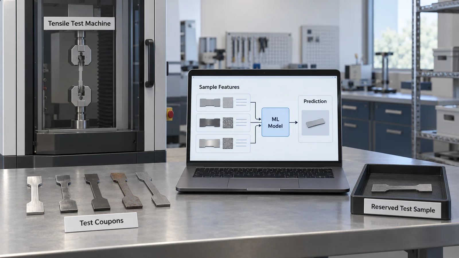
Machine learning fits a relationship between inputs and outputs to data. A neural network is one way of doing it: a stack of layered functions whose parameters are nudged, step by step, along the gradient of a loss. But fitting the training data and being right on a new sample are two different things. This article walks through the three types of learning, loss and optimisation, backpropagation, overfitting and the basics of evaluation, checking each with a small numerical example. The second half is for materials engineers who use these methods on their own data or research, and covers the usual traps (data leakage, extrapolation, small datasets), within what primary sources support.
- What machine learning is (the short version)
- Three types of learning — supervised, unsupervised, reinforcement
- Model, loss, optimisation — how a neural network "learns"
- Backpropagation — following a small numerical example
- Generalisation and overfitting — fitting the training data versus being right on new data
- Evaluation basics — how to split the data, and which metric
- Cautions for materials engineers — leakage, extrapolation, small datasets
- Where compute comes in — parameter count and memory
- Limits, and what could not be confirmed / Summary
- How to read evaluations and standards
- Glossary
- References
- Claim-to-source audit
Sourced = stated in published material (link given)
Our calculation = a figure this article derived, with the assumptions spelled out
Not yet confirmed = under revision, in preparation or at the proposal stage, so not final
Readings for materials research are marked separately as Commentary. Inference is shown in bold.
The numerical examples in Sections 4 to 6 are calculations on small synthetic datasets that we generated (with a fixed random seed). They do not describe any real materials dataset or product. They are not recipes ("do this and it works"); they are there to show mechanisms and pitfalls in numbers. For the ISO/IEC standards we checked titles and scope only, not the texts. We do not rank particular software or companies.
1. What machine learning is (the short version)
- Machine learning means fitting a function to data. Instead of writing a formula by hand that maps inputs (composition, an image, a spectrum) to an output (a property value, a defect or no defect), you adjust parameters to the data.
- A neural network is linear transformations and nonlinear functions stacked in layers. Every parameter is moved a little in the direction that lowers the loss (the gap between prediction and answer). The direction for each parameter is found efficiently by backpropagation Sourced [Ref. 1].
- A good fit on the training data does not guarantee a good fit on new samples. What tends to break an evaluation is how the data are split (samples from the same family straddling training and evaluation: "leakage"), the choice of metric, and extrapolating beyond the range of the training data.
Fitting the training data is not evidence that a model will be right on new data. Zhang et al. showed that neural networks for image recognition can fit training data easily (they can drive the training error down) even when the labels have been replaced with random ones Sourced [Ref. 5]. Fitting alone can be achieved without learning anything.
2. Three types of learning — supervised, unsupervised, reinforcement
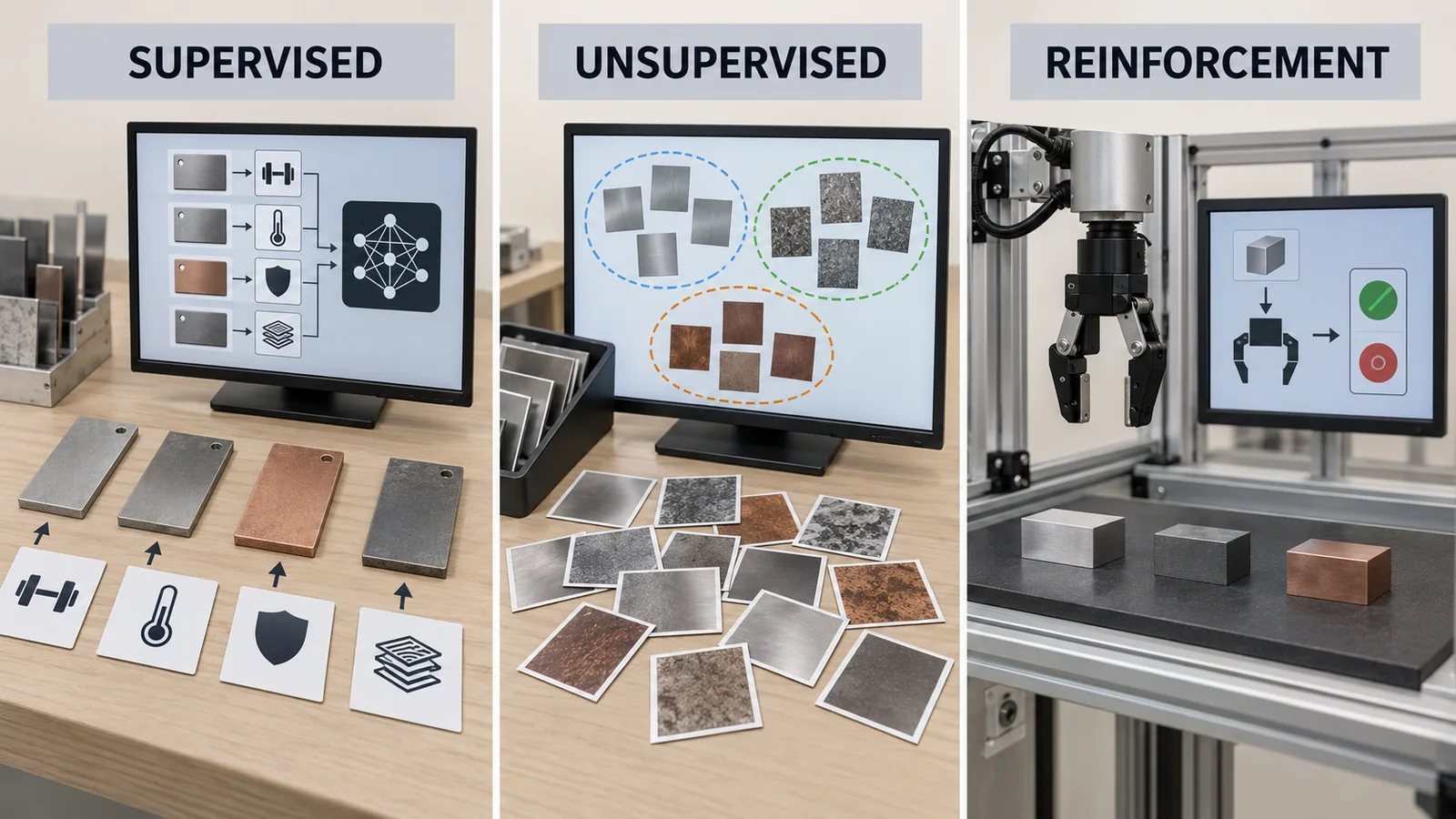
For this introduction, we organise learning goals as reducing error against targets, learning representations without target labels, and learning a policy from actions and rewards. This is our introductory organisation, not a claim that every method belongs in exactly one box. The original backpropagation study [Ref. 1], the individual studies below and official implementation documentation support the specific mechanisms and evaluations discussed here.
| Type | Data supplied | Goal of learning | Example uses in materials work (commentary) | Caution |
|---|---|---|---|---|
| Supervised learning | Pairs of an input x and its correct answer y | Build a function that returns y from x. Regression (continuous values) and classification (categories) | Predict a property value from composition or structure; classify defects in micrographs | The quality and cost of the labels y are the constraint. Measurement scatter sets a floor under prediction error |
| Unsupervised learning | Inputs x only (no answers) | Find structure in the data: groupings, or a representation on a few axes | Clustering of spectra or micrographs; dimensionality reduction for visualisation | With no "answer", quality has to be judged separately for each purpose |
| Reinforcement learning | Interaction with an environment (actions and the resulting states and rewards) | Find a policy that raises the cumulative reward | Described as a framework for changing conditions step by step to raise a reward (a target metric). We did not confirm practical examples in materials work | The reward design decides the outcome. Each trial is costly |
The three categories and the materials examples are our introductory organisation, not an experimental result.
View original SVG, values and source annotations
The core of large language model training is self-supervised learning, where the labels are made from the data itself (for example, predicting the next word in a text). We cover it in our explainer on Transformers and large language models. The later stage that adjusts a model with human preferences as a reward (an application of reinforcement learning) is covered in our explainer on post-training and fine-tuning.
3. Model, loss, optimisation — how a neural network "learns"
(1) The model: linear transformations and nonlinear functions stacked up
One layer of a neural network multiplies an input vector x by a weight matrix W, adds a bias b, and passes the result through an activation function φ such as tanh or ReLU (h = φ(Wx + b)). Stacking many such layers gives the network. Because the activation is nonlinear, stacking layers lets the network represent curved functions (this article's commentary). Hornik et al. established the "universal approximation" result: a standard multilayer feedforward network with a hidden layer can approximate functions to any desired accuracy if it has enough hidden units Sourced [Ref. 3]. But this is a statement that a network that approximates the function exists. It does not guarantee that the parameters can be found from data, or that the network will be right on new data (commentary). We did not check the finer conditions of the theorem (the type of activation, the sense of approximation) against the body of the original paper.
(2) The loss: turning "error" into a single number
The loss function L puts the goal of learning into a formula. Regression commonly uses the mean of the squared differences between prediction and answer (mean squared error); classification uses cross-entropy, based on the logarithm of the probability given to the correct class (this article's explanation). The loss is part of the design that decides "what counts as good", and it can be chosen separately from the evaluation metric.
(3) Optimisation: moving the parameters along the gradient
Gradient descent moves the parameters θ in the direction that lowers the loss (the opposite of the gradient), by a step set by the learning rate η (θ ← θ − η∇L). Stochastic gradient descent (SGD) estimates the gradient from a small subset of the data (a mini-batch) rather than all of it. Adam keeps moving averages of the first and second moments of the gradient and adjusts the step per parameter. The original paper gives, as good default settings for the problems it tested, α = 0.001, β1 = 0.9, β2 = 0.999 and ε = 10−8 Sourced [Ref. 2]. These are defaults for the problems in that paper, not values that are best for every dataset (commentary). Hyperparameters such as the learning rate, batch size and the number and width of layers are chosen on validation data, not training data (Section 6).
| One step of training | What happens | Caution |
|---|---|---|
| 1. Forward pass | Feed in a mini-batch and pass it through the layers to get the predictions ŷ | Intermediate values from each layer are stored for the backward pass (this uses memory) |
| 2. Loss | Turn the gap between prediction and answer into the loss L | The definition of the loss decides what counts as good |
| 3. Backward pass | Compute the gradient of L with respect to each parameter, from the output side backwards | See the numerical example in Section 4 |
| 4. Update | Move the parameters using the gradient and an optimiser (SGD, Adam, and so on) | Too large a learning rate diverges; too small a rate makes little progress |
| 5. Repeat | Go through the data several times (epochs) while watching the loss on validation data | If the validation loss starts to worsen, countermeasures such as stopping early are available |
The training loop is our explanation of calculating a loss and using gradients to update parameters. It is not the complete workflow of a particular implementation.
An example of counting parameters (Our calculation): a fully connected network with 784 inputs, 128 hidden units and 10 outputs (a shape often used for handwritten-digit classification) has 784×128 + 128 + 128×10 + 10 = 101,770 parameters. One forward pass costs about 2 × 101,770 ≈ 200,000 floating-point operations (counting a multiply and an add together as 2, and leaving out activations and similar terms).
4. Backpropagation — following a small numerical example
Backpropagation is the learning procedure reported by Rumelhart, Hinton and Williams in 1986 [Ref. 1]. Starting from a loss that expresses the difference between outputs and targets, it computes backwards how to adjust the weights in each layer. The equations and small numerical example below are our explanation of this procedure.
The mechanism is the chain rule (differentiating composed functions). Starting from "how sensitive the loss is to the output" at the output side, and multiplying back through one layer at a time, gives the gradients for all parameters at a cost of roughly the same order as the forward pass (this article's commentary). The example below is a network with two inputs, two hidden units (tanh) and one output.
- Input x = (1, 2); weights W₁ = [[0.1, 0.2], [0.3, 0.4]] and W₂ = (0.5, 0.6); biases 0; target t = 1.
- The forward pass gives ŷ = 0.7114 and loss L = 0.04166. The backward pass gives, for one component of W₁, ∂L/∂W₁[0,0] = −0.11350.
- Whether this gradient is right can be checked by numerical differentiation: move the weight by a tiny amount (10−6) and measure the change in loss. Our calculation gives −0.113501, matching the backpropagation value (−0.113501).
- One update at learning rate 0.1 lowers the loss from 0.04166 to 0.02759.
Our calculation. Python (NumPy), double precision. The inputs, weights and target are illustrative values, not real data.
To get each layer's gradient, backpropagation reuses the intermediate values from the forward pass (h in the example above). So training uses more memory than inference (prediction alone). As networks grow, these intermediate values, the parameters, the gradients and the optimiser state take up memory, and as Section 8 shows, memory capacity and bandwidth become the constraint on computation.
From a materials standpoint, this constraint is where the demands on HBM (high bandwidth memory) stacking, on packaging and on cooling materials come from. We cover this in our explainers on HBM and on AI accelerators (this article's commentary).
5. Generalisation and overfitting — fitting the training data versus being right on new data
The aim of learning is not to memorise the training data but to be right on data the model has not seen (generalisation). When a model is so complex that it fits even the noise in the data, that is overfitting; when it is too simple to capture even the trend, that is underfitting. The figure below reproduces overfitting on a small synthetic dataset.
- Data: the training set is 15 points of y = sin(2πx) with normal noise of standard deviation 0.2 added. For evaluation we used 2,000 new points made the same way (random seed 0).
- Model: polynomials (the higher the degree, the more freedom), fitted by least squares.
- Result: at degrees 1 and 2 the fit is close to a straight line and misses on both training and test data (underfitting). At degrees 3 to 5 the test error is lowest, about 0.24. As the degree rises further, the training error keeps falling while the test error climbs (0.41 at degree 9).
- Degree 14 (a curve through all 15 points): the training error is almost zero, but the test error jumps to about 8,600 (numerical precision also plays a part).
Our calculation. Synthetic data; not the result for any particular materials dataset. The measurement noise (0.2) is a rough floor that no model can get below (this article's commentary).
(1) Ways to curb overfitting (the general ones)
The usual methods are to add data, make the model smaller, regularise (penalise large weights, as in weight decay), stop early (halt when the validation loss starts to worsen), and use dropout (randomly disabling units during training). Srivastava et al. proposed dropout as a simple way of preventing overfitting in neural networks Sourced [Ref. 4]. The other methods are explained here as introductory terminology.
(2) "More complexity always makes things worse" is not always true
Classical statistics says that a model that is too complex has too much variance and the test error rises (a U-shaped curve). Yet modern neural networks are known to reach high accuracy even when large enough to interpolate the training data exactly. Belkin et al. reconciled the two in a double descent curve: past the point where the model can interpolate the data (the interpolation threshold), adding complexity makes performance better again Sourced [Ref. 6]. Nakkiran et al. showed that double descent occurs not only with model size but also with the number of training epochs, and that there are even regimes where more training data hurts performance Sourced [Ref. 7].
The polynomial example in the figure above (the classical U shape) and the double descent of very large neural networks are different phenomena, observed with different model types, data, regularisation and training methods (this article's commentary). What practice tells us is that "which complexity is best" cannot be decided from theory; you measure it on validation data and decide.
(3) Re-using the same evaluation set has limits too
If the same evaluation set is used for years, researchers may unconsciously choose models and settings to suit that set. Recht et al. rebuilt new test sets for CIFAR-10 and ImageNet by following the original creation procedures closely, and re-measured existing models. Accuracy fell by 3–15% on CIFAR-10 and by 11–14% on ImageNet Sourced [Ref. 8]. At the same time, gains in accuracy on the original test sets translated into larger gains on the new ones. The authors conclude that the drop is due not to adaptation to the evaluation data but to the models' inability to generalise to slightly "harder" images than those in the original test sets [Ref. 8].
The lesson is that a number on an evaluation set is conditioned on how that set was made and used (this article's commentary). Our explainer on benchmarks and how to read evaluations treats this at length for language-model benchmarks.
6. Evaluation basics — how to split the data, and which metric
(1) Training, validation and test sets
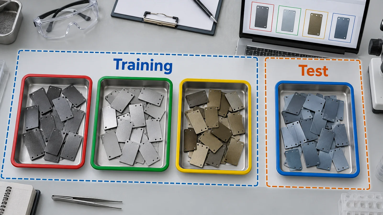
Split the data into a training set (to learn the parameters), a validation set (to choose hyperparameters and models) and a test set (used once at the end to report performance). When data are scarce, cross-validation is used: split into training and validation sets several ways and average. The scikit-learn user guide explains that a model which merely repeated the labels of samples it had just seen would score perfectly but be useless on unseen data, and that holding out part of the data as a test set is therefore the usual practice Sourced [Ref. 19].
(2) Choose the metric for the purpose
Metrics depend on the kind of output. Classification uses accuracy, precision, recall, the F1 score and the area under the ROC curve (AUC); regression uses mean absolute error (MAE), root-mean-square error (RMSE) and the coefficient of determination (R²) (this article's commentary). ISO/IEC TS 4213:2022 is a technical specification that sets out methods for measuring the classification performance of machine learning models, systems and algorithms Sourced [Ref. 23] (its text is paid, and we did not check it).
Example: classification for rare defects (Our calculation). Suppose 100 of 10,000 samples (1%) are defective. A do-nothing model that simply answers "good" for everything still has an accuracy of 99%. Now take a model that finds 60 of the 100 defective samples (recall 60%) but wrongly flags 140 of the 9,900 good ones (precision 60 ÷ 200 = 30%). Its accuracy is 98.2%, lower than the do-nothing model's. Its F1 score is 0.40.
| Model | True positives | False negatives | False positives | True negatives | Accuracy | Precision | Recall |
|---|---|---|---|---|---|---|---|
| Always answers "good" | 0 | 100 | 0 | 9,900 | 99.0% | undefined | 0% |
| A model that picks up defects (example) | 60 | 40 | 140 | 9,760 | 98.2% | 30% | 60% |
Our calculation. The numbers are an illustrative, hypothetical example. With imbalanced data, accuracy alone cannot tell you whether a model is any good. Which metric to use should be decided by the cost of misses (false negatives) and false alarms (false positives) (this article's commentary).
(3) Compare with a simple baseline
A complex model's number alone does not say whether it is good. It means something only when compared with a simple baseline, such as "always return the mean" or "return the value of the nearest training sample". Meredig et al. introduced a simple nearest-neighbour benchmark in evaluating machine learning for materials discovery Sourced [Ref. 11].
7. Cautions for materials engineers — leakage, extrapolation, small datasets
Materials data are often made up of families of samples (a series with the same composition, the same deposition batch, repeated measurements on the same tool), which makes the data split and the evaluation prone to pitfalls (this article's commentary).
(1) Data leakage
Kapoor and Narayanan report that, in the research communities that use machine learning, data leakage was found in 17 fields, affecting at least 294 papers. They sort leakage into eight types: no test set, pre-processing across training and test sets, feature selection across them, duplicated data, illegitimate features, temporal leakage, non-independence between training and test samples, and a test distribution that is biased Sourced [Ref. 10]. The typical case with materials data is the same sample, or samples from the same family, falling in both training and evaluation. This is Kapoor et al.'s "non-independence between train and test samples" (L3.2). As a remedy, they point to splits that respect the dependencies between training and test data (block cross-validation and the like) [Ref. 10, 13]. scikit-learn's GroupKFold is a way of splitting so that the same group never appears in both training and evaluation sets Sourced [Ref. 20].
The following experiment on synthetic data shows how the way of splitting changes the evaluation (Our calculation). We made 30 families of 10 samples each. The features of each family are a fixed pattern for that family plus small noise, and the property value is a family-specific value (standard deviation 2 between families) plus small noise (0.3). That property value is unrelated to the differences in features within a family. Running 5-fold cross-validation with a simple 3-nearest-neighbour predictor gives:
- Random split: coefficient of determination R² = 0.96 (samples of the same family are also in training, so simply copying the values of near neighbours scores high).
- Split by family: R² = −1.28 (the evaluation families are entirely absent from training, and the value for a new family cannot be predicted).
Our calculation. An extreme synthetic dataset (the property is set by the family alone). How far apart the two figures are for real data depends on the size of the family effect. R² can fall below 0 (worse than predicting the mean).
An evaluation number is the result of deciding, through the way you split the data, "what to call new data". Whether you want to know performance on a new composition, a new deposition batch or a new tool or a new day determines the unit (group) to split by. If you want performance on a new composition but repeat measurements of the same composition are also in the test set, the number will be inflated (this article's commentary).
Pre-processing (standardisation, feature selection) done on all the data up front is also one of Kapoor et al.'s leakage types [Ref. 10]. Pre-processing should also be learned from the training data only, and merely applied to the test data.
(2) Extrapolation: searching for new materials is usually an extrapolation problem
Meredig et al. state that "traditional machine learning metrics overestimate model performance for materials discovery". They introduced leave-one-cluster-out cross-validation (LOCO CV), which removes a whole cluster of similar materials at a time for evaluation, and a simple nearest-neighbour benchmark. They report that performance in discovery applications depends strongly on the problem, the data sampling and the extrapolation Sourced [Ref. 11]. If the aim is to search outside the range of the training data (a new chemical system, a new composition region), a number from a random split is not an evaluation that fits that aim (this article's commentary).
(3) Small datasets
Zhang and Ling noted that materials datasets are typically smaller, and sometimes more diverse, than in other fields, and studied the relation between data size and predictive performance. They found that the effect of data size is mediated by the degrees of freedom (DoF) of the model, and that the appearance of a precision-DoF association signals underfitting Sourced [Ref. 14]. Matbench, the benchmark for materials property prediction by Dunn et al., has 13 tasks ranging from 312 to 132,000 samples, and its authors report that crystal-graph methods appear to outperform traditional descriptor-based methods given roughly 104 or more data points Sourced [Ref. 12]. The reading (this article's commentary) is that the less data you have, the more the quality of the data, and the effort of building physical and chemical knowledge into the features, count for compared with the choice of model.
(4) Shortcut learning, and different models with the same score
Geirhos et al. tested CNNs and humans on images with conflicting texture and shape cues. They reported a texture bias in ImageNet-trained CNNs and showed that changing the training images could produce shape-based representations [Ref. 15]. This is a result for specific images and models, not a universal law. Our materials-image example is a caution to check whether a model relies on background rather than the specimen. For behaviour that changes across deployment settings, see the original study by D’Amour et al. [Ref. 16].
The dotted line in the figure of Section 5 is the size of the measurement noise. No model can achieve errors far below it (a training error below that level is a sign that the model has memorised the noise, that is, overfitting). If you know beforehand how much repeat measurements of the same sample scatter (repeatability), that gives a yardstick for whether a model is good enough (this article's commentary).
Also, the output of an ordinary neural network is a single value (a point estimate) with no indication of how reliable it is. Ensembles, which average several models, have been reported as one simple way of estimating predictive uncertainty Sourced [Ref. 17]. When choosing the next sample to measure in a materials search, an estimate of uncertainty, not just the predicted value, informs the decision (this article's commentary).
Combining machine learning with materials search and automated experiments is covered in our "Materials Informatics" field. This article limits itself to the groundwork and to the pitfalls of evaluation.
8. Where compute comes in — parameter count and memory
Small networks, and machine learning on materials features, can often be trained on a laptop in seconds to minutes, so the constraint from computing resources is small (this article's commentary). For models with billions of parameters or more, on the other hand, memory is the first constraint.
The ZeRO paper explains that when training with Adam in mixed precision (computing in half precision, fp16, and keeping an fp32 copy), each parameter needs 2 bytes for the parameter (fp16), 2 bytes for the gradient (fp16) and 12 bytes of optimiser state (the fp32 copy of the parameter, the first moment and the second moment), 16 bytes in all Sourced [Ref. 18]. For a model with Ψ parameters, that is 16Ψ bytes. From this we can compute a lower bound on memory for each model size.
| Parameters | Parameters, gradients and optimiser state combined (16 bytes each) | How to read it |
|---|---|---|
| 100 million (108) | 1.6 GB | Fits comfortably in the memory of a single GPU |
| 1 billion (109) | 16 GB | Takes up a large share of one GPU's memory |
| 7 billion (7×10⁹) | 112 GB | A scale beyond the memory of a single GPU; it has to be spread over several |
Our calculation. 16Ψ bytes is the mixed-precision Adam case in the ZeRO paper [Ref. 18]. Activations (intermediate values kept for backpropagation), batch size and communication buffers are not included (real requirements are larger). GPU memory capacity differs by product and generation, so no particular product's figure is used here.
This constraint leads to demands on HBM (high bandwidth memory) stacking, on 2.5D packaging such as CoWoS, and on thermal interface materials to carry heat away. We treat these in our explainers on HBM, CoWoS, thermal interface materials (TIM) and AI accelerators.
9. Limits, and what could not be confirmed / Summary
(1) The texts of the standards
The texts of ISO/IEC 22989, 23053, TS 4213, 5259-1, 5259-3, 23894 and 42001 are paid, and we did not check them. This article limits itself to the numbers, titles, publication dates and stages shown on the ISO pages, and states no requirements or definitions.
(2) The numbers from synthetic data
The numbers in Sections 4 to 7 come from calculations on synthetic data that we generated. The errors by degree, the gap between R² values and the confusion-matrix example are there to show mechanisms; they do not indicate the size of the effects in real materials data.
(3) The conditions of universal approximation
For the result of Hornik et al. we kept to the title and the general understanding. We did not check finer details, such as the conditions on the activation function and the sense of approximation, against the body of the original paper.
(4) Methods not covered
We do not cover decision trees, random forests and gradient boosting, support vector machines, Gaussian-process regression, or convolutional, recurrent and graph neural networks. These are probably also widely used on tabular materials data, but we did not check primary sources for that. Transformers are covered in our explainer on Transformers and large language models.
(5) Practical use of reinforcement learning in materials and process work
We did not confirm practical examples of reinforcement learning in materials or process work.
- Machine learning fits parameters to data. A neural network learns a layered function by the gradient of a loss, found with backpropagation Sourced
- Fitting the training data is not evidence of generalisation. Networks can fit random labels. In the synthetic example, the training error kept falling as the degree rose while the test error rose Sourced / Our calculation
- Choose the metric for the purpose. In a search for rare defects, a do-nothing model's accuracy (99%) can exceed that of a useful model (98.2%) Our calculation
- Materials data are made of families of samples. If a family straddles training and evaluation, the number is inflated (R² of 0.96 versus −1.28 on synthetic data). Searching for new materials is extrapolation, and small datasets need care too Sourced / Our calculation
- For large models, the first constraint is memory. Mixed-precision Adam needs 16 bytes of state per parameter Sourced
10. How to read evaluations and standards
The performance of machine learning becomes a number only once you fix the evaluation data, how the data are split, the metric and the baseline for comparison. Classification is measured by metrics computed from the confusion matrix, regression by error metrics, and methods are compared on shared research benchmarks (ImageNet, Matbench and others). Safety and reliability need more than a number: standards and guidance (ISO/IEC, NIST) cover data quality, risk management and how an organisation operates. The table below sets out what we could confirm (checked 15 October 2026).
| What is evaluated | Representative benchmarks and methods (name, source) | Standards and guidance (ISO/IEC, NIST and others) | Cautions in reading |
|---|---|---|---|
| Classification performance | Metrics based on the confusion matrix (accuracy, precision, recall, F1). Section 6 Our calculation | ISO/IEC TS 4213:2022 "Information technology — Artificial intelligence — Assessment of machine learning classification performance" (published October 2022; the ISO page shows it at the "to be revised" stage) [26] Sourced Not yet confirmed | With imbalanced data, accuracy misleads. Choose the metric by the cost of misses and false alarms |
| Generalisation | Hold-out and cross-validation (scikit-learn user guide) [22]. Re-measurement on a new test set (Recht et al., 2019) [11] Sourced | ISO/IEC 23053:2022 "Framework for Artificial Intelligence (AI) Systems Using Machine Learning (ML)" (published June 2022) [25]. We did not check what evaluation procedures it contains Sourced | Re-use of the evaluation set and the way the data are split change the number (Sections 5 and 7) |
| Research benchmark for image classification | ImageNet Large Scale Visual Recognition Challenge (1,000 categories; Russakovsky et al., 2015) [12]. New test sets (Recht et al.) [11] Sourced | Could not be confirmed | Even on the same data, a comparison is conditioned on how the evaluation data were made and used |
| Prediction of materials properties | Matbench (13 tasks, 312 to 132,000 samples; Dunn et al., 2020) [15]. Leave-one-cluster-out cross-validation and a nearest-neighbour benchmark (Meredig et al., 2018) [14] Sourced | Could not be confirmed | A random split makes extrapolation performance look better than it is. Measure with splits by family or cluster |
| Quality of training data | Could not be confirmed (we did not find a common benchmark for dataset quality) | ISO/IEC 5259-1:2024 (data quality: overview, terminology and examples) and ISO/IEC 5259-3:2024 (data quality management: requirements and guidelines). The ISO page lists the 5259 series as a package of five parts [27, 28] Sourced | We did not check the texts, so we state no requirements |
| Concepts and terminology | (Not an evaluation: a terminology standard) | ISO/IEC 22989:2022 "Artificial intelligence concepts and terminology" (published July 2022) [24] Sourced | Definitions can differ in detail between sources (textbooks, standards) |
| Risk management and operation | — | ISO/IEC 23894:2023 (guidance on AI risk management) [29] and ISO/IEC 42001:2023 (AI management systems) [30]. NIST AI RMF 1.0 (NIST AI 100-1, January 2023; voluntary use) [31] Sourced | We found no successor to NIST AI RMF as of the checking date. We did not check the requirements of ISO/IEC 42001 |
| Reproducibility and leakage checks | Model info sheets (Kapoor and Narayanan, 2023), which ask for an account of splits, pre-processing, duplicates and so on for each of the eight leakage types [13] Sourced | Could not be confirmed | Some leakage cannot be found by reading a paper. Reports should state the unit of the split and the pre-processing steps |
The arrangement of the table is Our calculation (organisation). The numbers, titles, dates and stages of ISO/IEC standards were checked on the official ISO pages (checked 15 October 2026). The texts of the standards are paid, so we limit ourselves to their scope.
Cautions in reading (for materials engineers)
- Numbers change with settings and with who ran the evaluation: R² and accuracy change with the unit of the data split, the order of pre-processing and who evaluated (the developer or a third party). Do not rank figures obtained under different settings against each other just because the metric has the same name.
- An evaluation set wears out with re-use: when the same evaluation set is used for a long time, the numbers can reflect adaptation to that set, or quirks peculiar to how it was made [Ref. 8, 15].
- Most standards and guidance are voluntary: ISO/IEC standards generally gain binding force only when cited in law or contract, and NIST AI RMF is intended for voluntary use [Ref. 28] (the general position of ISO/IEC standards is this article's commentary). When someone says "compliant with a standard", check which requirements of which standard they mean.
- Stated values and measured values are different: an accuracy in a paper or catalogue is a value from a conditioned experiment. It is worth re-measuring on your own data with your own split.
11. Glossary
- Supervised learning
- Learning a function from inputs to outputs using pairs of inputs and correct answers.
- Unsupervised learning
- Finding groupings or a few axes in data that have no answers.
- Reinforcement learning
- Learning a policy of actions that raises cumulative reward through interaction with an environment.
- Loss function
- The gap between prediction and answer expressed as one number. Learning makes it smaller.
- Gradient descent / SGD
- Moving parameters in the direction that lowers the loss. SGD estimates the gradient from mini-batches.
- Adam
- An optimiser that adjusts the step per parameter using first and second moments of the gradient.
- Backpropagation
- The procedure that computes the gradient of the loss from the output side backwards using the chain rule.
- Activation function
- A function that gives a layer's output its nonlinearity (tanh, ReLU and so on).
- Overfitting / underfitting
- Fitting even the noise in the training data / failing to capture even the trend.
- Generalisation
- Being right on data not yet seen.
- Regularisation
- Measures such as penalising complexity to curb overfitting.
- Cross-validation
- Splitting the data several ways, training and evaluating each time, and averaging.
- Data leakage
- Information that should be reserved for evaluation getting into training. It inflates the evaluation.
- Precision / recall
- The share of positive calls that are correct / the share of true positives that were found.
- LOCO CV
- Cross-validation that removes a whole cluster of similar items at a time. Used to evaluate extrapolation.
- Hyperparameter
- A setting chosen by people before training, such as the learning rate or number of layers.
- Double descent
- The phenomenon where performance that worsens as complexity grows improves again with further complexity.
- Shortcut learning
- Using decision rules that do well on standard tests but do not carry over to real conditions.
12. References
- Rumelhart D. E., Hinton G. E., Williams R. J. "Learning representations by back-propagating errors", Nature 323, 533–536 (1986), DOI 10.1038/323533a0 — nature.com/articles/323533a0
- Kingma D. P., Ba J. "Adam: A Method for Stochastic Optimization", arXiv:1412.6980 (ICLR 2015) — arxiv.org/abs/1412.6980
- Hornik K., Stinchcombe M., White H. "Multilayer feedforward networks are universal approximators", Neural Networks 2, 359–366 (1989), DOI 10.1016/0893-6080(89)90020-8 — doi.org/10.1016/0893-6080(89)90020-8
- Srivastava N. et al. "Dropout: A Simple Way to Prevent Neural Networks from Overfitting", J. Mach. Learn. Res. 15, 1929–1958 (2014) — jmlr.org/papers/v15/srivastava14a.html
- Zhang C. et al. "Understanding deep learning requires rethinking generalization", arXiv:1611.03530 (ICLR 2017) — arxiv.org/abs/1611.03530
- Belkin M. et al. "Reconciling modern machine-learning practice and the classical bias–variance trade-off", Proc. Natl. Acad. Sci. USA 116, 15849–15854 (2019), DOI 10.1073/pnas.1903070116 — doi.org/10.1073/pnas.1903070116
- Nakkiran P. et al. "Deep Double Descent: Where Bigger Models and More Data Hurt", arXiv:1912.02292 — arxiv.org/abs/1912.02292
- Recht B. et al. "Do ImageNet Classifiers Generalize to ImageNet?", arXiv:1902.10811 (ICML 2019) — arxiv.org/abs/1902.10811
- Russakovsky O. et al. "ImageNet Large Scale Visual Recognition Challenge", Int. J. Comput. Vis. 115, 211–252 (2015), DOI 10.1007/s11263-015-0816-y — doi.org/10.1007/s11263-015-0816-y
- Kapoor S., Narayanan A. "Leakage and the reproducibility crisis in machine-learning-based science", Patterns 4, 100804 (2023), DOI 10.1016/j.patter.2023.100804 (open access) — doi.org/10.1016/j.patter.2023.100804
- Meredig B. et al. "Can machine learning identify the next high-temperature superconductor? Examining extrapolation performance for materials discovery", Mol. Syst. Des. Eng. 3, 819–825 (2018), DOI 10.1039/C8ME00012C — doi.org/10.1039/C8ME00012C
- Dunn A. et al. "Benchmarking materials property prediction methods: the Matbench test set and Automatminer reference algorithm", npj Comput. Mater. 6, 138 (2020), DOI 10.1038/s41524-020-00406-3 (open access) — doi.org/10.1038/s41524-020-00406-3
- Roberts D. R. et al. "Cross-validation strategies for data with temporal, spatial, hierarchical, or phylogenetic structure", Ecography 40, 913–929 (2017), DOI 10.1111/ecog.02881 — doi.org/10.1111/ecog.02881
- Zhang Y., Ling C. "A strategy to apply machine learning to small datasets in materials science", npj Comput. Mater. 4, 25 (2018), DOI 10.1038/s41524-018-0081-z (open access) — doi.org/10.1038/s41524-018-0081-z
- Geirhos R. et al. "ImageNet-trained CNNs are biased towards texture; increasing shape bias improves accuracy and robustness", ICLR 2019, arXiv:1811.12231 — https://arxiv.org/abs/1811.12231
- D'Amour A. et al. "Underspecification Presents Challenges for Credibility in Modern Machine Learning", arXiv:2011.03395 — arxiv.org/abs/2011.03395
- Lakshminarayanan B., Pritzel A., Blundell C. "Simple and Scalable Predictive Uncertainty Estimation using Deep Ensembles", arXiv:1612.01474 (NeurIPS 2017) — arxiv.org/abs/1612.01474
- Rajbhandari S. et al. "ZeRO: Memory Optimizations Toward Training Trillion Parameter Models", arXiv:1910.02054 (SC20) — arxiv.org/abs/1910.02054
- scikit-learn User Guide, "Cross-validation: evaluating estimator performance" — scikit-learn.org/stable/modules/cross_validation.html
- scikit-learn API, "GroupKFold" — scikit-learn.org/.../sklearn.model_selection.GroupKFold.html
- ISO/IEC "ISO/IEC 22989:2022 Information technology — Artificial intelligence — Artificial intelligence concepts and terminology" (ISO page) — iso.org/standard/74296.html
- ISO/IEC "ISO/IEC 23053:2022 Framework for Artificial Intelligence (AI) Systems Using Machine Learning (ML)" (ISO page) — iso.org/standard/74438.html
- ISO/IEC "ISO/IEC TS 4213:2022 Information technology — Artificial intelligence — Assessment of machine learning classification performance" (ISO page) — iso.org/standard/79799.html
- ISO/IEC "ISO/IEC 5259-1:2024 Artificial intelligence — Data quality for analytics and machine learning (ML) — Part 1: Overview, terminology, and examples" (ISO page) — iso.org/standard/81088.html
- ISO/IEC "ISO/IEC 5259-3:2024 Artificial intelligence — Data quality for analytics and machine learning (ML) — Part 3: Data quality management requirements and guidelines" (ISO page) — iso.org/standard/81092.html
- ISO/IEC "ISO/IEC 23894:2023 AI — Guidance on risk management" (ISO page) — iso.org/standard/77304.html
- ISO/IEC "ISO/IEC 42001:2023 AI management systems" (ISO page) — iso.org/standard/81230.html
- NIST "Artificial Intelligence Risk Management Framework (AI RMF 1.0)", NIST AI 100-1, January 2023, DOI 10.6028/NIST.AI.100-1 — doi.org/10.6028/NIST.AI.100-1
13. Claim-to-source audit
| Claim in the text | Basis | Class |
|---|---|---|
| Backpropagation was reported as a procedure that repeatedly adjusts connection weights to minimise a measure of the difference between actual and desired output, with hidden units coming to represent features of the task (Rumelhart et al., 1986) | Nature article page (abstract) Reference 1 https://www.nature.com/articles/323533a0 | Sourced |
| The Adam defaults (α=0.001, β₁=0.9, β₂=0.999, ε=10⁻⁸) are given as good defaults for the problems tested | Kingma and Ba (note to Algorithm 1) Reference 2 https://arxiv.org/abs/1412.6980 | Sourced |
| The result that multilayer feedforward networks are universal function approximators (title). Details of the conditions were not checked | Title and bibliographic details of Hornik et al. (1989) Reference 3 https://doi.org/10.1016/0893-6080(89)90020-8 | Sourced |
| Dropout was proposed as a simple way to prevent overfitting in neural networks | Title of Srivastava et al. (2014) Reference 4 https://jmlr.org/papers/v15/srivastava14a.html | Sourced |
| Networks can easily fit random labels | Zhang et al. (2017) Reference 5 https://arxiv.org/abs/1611.03530 | Sourced |
| The double descent curve subsumes the classical U shape; double descent with model size and epochs, and the regime where more training data worsens performance | Belkin et al. (2019); Nakkiran et al. Reference 6 https://doi.org/10.1073/pnas.1903070116 Reference 7 https://arxiv.org/abs/1912.02292 | Sourced |
| On new test sets, accuracy fell by 3–15% on CIFAR-10 and 11–14% on ImageNet; gains on the original sets translated into larger gains on the new ones; the authors' conclusion that the cause is not adaptation to the evaluation data but an inability to generalise to slightly harder images | Abstract and introduction of Recht et al. (2019) Reference 8 https://arxiv.org/abs/1902.10811 | Sourced |
| ILSVRC is a benchmark with hundreds of object categories and millions of images, run annually from 2010, with more than fifty participating institutions; 1,000 categories | Russakovsky et al. (2015) Reference 9 https://doi.org/10.1007/s11263-015-0816-y | Sourced |
| Data leakage affected at least 294 papers in 17 fields; the eight leakage types; model info sheets | Kapoor and Narayanan (2023) Reference 10 https://doi.org/10.1016/j.patter.2023.100804 | Sourced |
| Traditional ML metrics overestimate performance for materials discovery; introduction of LOCO CV and a nearest-neighbour benchmark; performance depends on the problem, data sampling and extrapolation | Abstract of Meredig et al. (2018) Reference 11 https://doi.org/10.1039/C8ME00012C | Sourced |
| Matbench has 13 tasks (312 to 132,000 samples, 10 sources); crystal-graph methods appear to outperform traditional methods at roughly 10⁴ or more data points | Abstract of Dunn et al. (2020) Reference 12 https://doi.org/10.1038/s41524-020-00406-3 | Sourced |
| With structured data, random cross-validation underestimates prediction error, and block cross-validation can address it | Abstract of Roberts et al. (2017) Reference 13 https://doi.org/10.1111/ecog.02881 | Sourced |
| With small materials datasets, the effect of data size is mediated by model degrees of freedom, and a precision-DoF association signals underfitting | Abstract of Zhang and Ling (2018) Reference 14 https://doi.org/10.1038/s41524-018-0081-z | Sourced |
| Texture bias and the effect of changing training images in the tested CNN experiments; a result limited to those settings. | Geirhos et al., ICLR 2019 Reference 15 https://arxiv.org/abs/1811.12231 | Original study |
| Predictors treated as equivalent on training-domain performance can behave very differently when deployed (underspecification) | D'Amour et al. Reference 16 https://arxiv.org/abs/2011.03395 | Sourced |
| Ensembles were proposed as a simple and scalable way to estimate predictive uncertainty | Abstract of Lakshminarayanan et al. Reference 17 https://arxiv.org/abs/1612.01474 | Sourced |
| Mixed-precision Adam needs 2 bytes of parameter, 2 bytes of gradient and 12 bytes of optimiser state, 16Ψ bytes in all | ZeRO paper (section 3 discussion) Reference 18 https://arxiv.org/abs/1910.02054 | Sourced |
| The general practice of holding out a test set; GroupKFold as a split that keeps a group out of both training and evaluation | scikit-learn documentation Reference 19 https://scikit-learn.org/stable/modules/cross_validation.html Reference 20 https://scikit-learn.org/stable/modules/generated/sklearn.model_selection.GroupKFold.html | Sourced |
| Numbers, titles and publication dates of ISO/IEC 22989:2022 (July 2022), 23053:2022 (June 2022) and TS 4213:2022 (October 2022, at the "to be revised" stage) | ISO pages Reference 21 https://www.iso.org/standard/74296.html Reference 22 https://www.iso.org/standard/74438.html Reference 23 https://www.iso.org/standard/79799.html | Sourced |
| Numbers, titles and publication dates of ISO/IEC 5259-1:2024 and 5259-3:2024 (both July 2024), 23894:2023 (February 2023) and 42001:2023 (December 2023) | ISO pages Reference 24 https://www.iso.org/standard/81088.html Reference 25 https://www.iso.org/standard/81092.html Reference 26 https://www.iso.org/standard/77304.html Reference 27 https://www.iso.org/standard/81230.html | Sourced |
| NIST AI RMF 1.0 (NIST AI 100-1, January 2023) is intended for voluntary use, and a review is expected no later than 2028 | Text of NIST AI 100-1 Reference 28 https://doi.org/10.6028/NIST.AI.100-1 | Sourced |
| The error table by polynomial degree (1 to 14), the backpropagation example, the 99% versus 98.2% accuracy comparison, R² of 0.96 and −1.28, 101,770 parameters, and the memory table (1.6 GB, 16 GB, 112 GB) | Our calculation (Python, NumPy; synthetic data, fixed random seeds; the memory table uses the 16Ψ bytes of the ZeRO paper). Not results on real data | Our calculation |
| The texts of ISO/IEC standards (requirements, definitions, evaluation procedures), the conditions of the Hornik et al. theorem, practical use of reinforcement learning in materials work, other methods such as decision trees, and a successor to NIST AI RMF | Could not be confirmed in the primary sources accessible within the scope of this survey, so they are not stated | Commentary |
| The readings that "backpropagation remembers intermediate values", "what counts as new is set by the unit of the split", "measurement scatter sets the limit of prediction" and "ISO/IEC standards are mostly voluntary", and the example uses in materials work | This article's arrangement and commentary based on published content. Not views stated by any institution | Commentary |
| That Figs. 2, 3, 4 and 5 are explanatory drawings, not real observations or data, and that Figs. 1 and 6 are ImageGen-generated conceptual illustrations | Note by this article | Commentary |
Last updated 15 October 2026. Sources are limited to primary material (peer-reviewed papers, arXiv papers, and ISO and NIST official pages). The texts of ISO/IEC standards are paid and could not be checked. The numerical examples are calculations on synthetic data that we generated, not results on real materials data. The texts of ISO/IEC standards, the finer conditions of the universal approximation theorem, practical use of reinforcement learning in materials work, and other methods such as decision trees could not be confirmed and are not stated here. All figures are explanatory concept graphics or drawings that include our calculations. Figs. 1 and 6 are ImageGen-generated conceptual illustrations, and none of them shows a real cross-section, micrograph or physical product.