Machine-Learning Interatomic Potentials Explained

TECHNOLOGY EXPLAINER

Machine-Learning Interatomic Potentials
Near first-principles accuracy, far faster, but only inside the range they learned

The result of a molecular dynamics (MD) run depends on how the forces between atoms are set. Empirical force fields are fast but cover only limited materials. First-principles calculation (DFT) is accurate but heavy, and cannot handle long times or large systems. A machine-learning interatomic potential (MLIP) uses first-principles results as teachers to build "an approximator that returns energy and forces from an arrangement of atoms". This article explains how it works, how MACE, M3GNet, CHGNet and the universal (foundation) models differ, how to read accuracy numbers, and what happens outside the range the model learned, with a small experiment of our own. We do not decide which model is better.

Sources: papers by Behler and Parrinello, Bartók et al., Chen and Ong, Deng et al., Batatia et al., Riebesell et al., Fu et al., Loew et al. and others (Phys. Rev. Lett., Nature-family journals, npj Computational Materials, arXiv); official GitHub, Hugging Face and Matbench Discovery pages; and documents from CEN and NIST. Numerical examples are our own calculations. Checked on 22 October 2026

Fig. 1. Conceptual illustration generated with ImageGen. 1 reference calculations, 2 a learned force model, 3 particle dynamics. Faster evaluation does not establish validity outside the training domain.Not an actual product, facility or measurement. Enlarged models, lines, arrows and colours are explanatory.

Contents

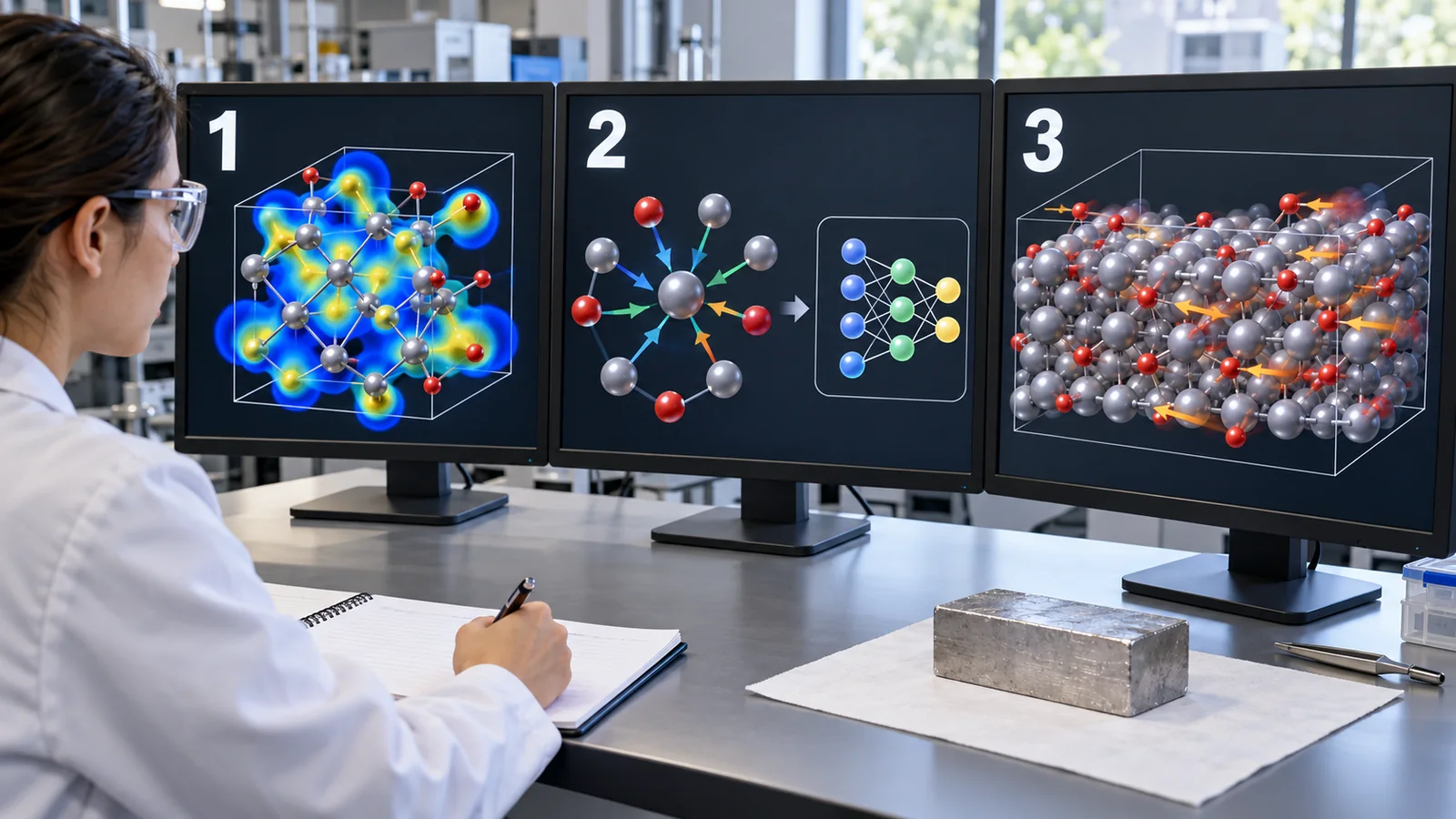
The short version, what to know first, and where this fits in the series
Why it is needed: DFT is accurate but heavy, empirical force fields are fast but narrow
How it works: from environment to per-atom energy, and then to forces
The main models and the universal (foundation) models
What "near first-principles accuracy" and "orders of magnitude faster" mean
How to read accuracy numbers
Cautions in use: outside the learned range
How to use one: as is, fine-tuned, or dedicated
A materials engineer's view
Limits, what we could not confirm, and a summary
How to read the yardsticks and standards
Glossary
References
Claim-to-source audit

Labels used in this article

Sourced = stated in a published source (linked)
Our calculation = a value computed in this article from the stated assumptions
Not yet confirmed = plans, targets, drafts, work in progress, outlooks: not settled
Our own reading for materials engineers is marked as commentary. Inference is shown in bold. Announcements by research groups and companies are labelled as the authors' claims.

1. The short version, what to know first, and where this fits in the series

An MLIP is an approximator that learns the map "atomic arrangement → energy and forces" from first-principles (DFT) data. The papers say it is orders of magnitude faster than DFT (Behler and Parrinello, 2007) Sourced[Ref. 1]
The ceiling on accuracy is the DFT it learned from. And it goes wrong outside the range it learned. In our small experiment, the largest error inside the range was 0.009, yet on the wall side the prediction was −0.27 where the true value was 1.96 Our calculation
Universal (foundation) models try to cover a wide part of the periodic table with one model. But the papers themselves state limits (short range only, no magnetic or spin degrees of freedom, and so on) Sourced[Ref. 12]. Because evaluation conditions differ, this article does not decide which model is better

What to know before reading

The prerequisites are that "the force between atoms comes from the slope of an energy surface" and that "MD moves atoms a little at a time with that force" (see our explainer on molecular dynamics). DFT is a physics simulation that computes the energy of matter from the behaviour of electrons; it contains approximations and does not always agree with measurement (see our explainer on density functional theory). This article is readable on its own.

The ideas shared across this series: machine learning is "an approximator that learns trends from past data", and it is weak outside the range of the data (extrapolation). It does not understand the laws of physics. Searching for materials is looking for buried treasure on a vast map; computation "proposes candidates quickly and cheaply", experiment "checks whether it is really so", and AI "narrows where to look". An MLIP is a tool for making "computation" faster.

Where this fits in the series

We suggest reading it after our explainers on molecular dynamics (how forces are used) and on density functional theory (how the training data are made). The reliability of MLIP results is covered in our explainers on uncertainty and applicability domains and on reading the evaluation and reproducibility of MI results. Searching crystal structures with MLIPs continues in our explainer on crystal structure prediction and stability, and generating candidates in our explainer on generative AI for materials design.

2. Why it is needed: DFT is accurate but heavy, empirical force fields are fast but narrow

To move atoms in MD you need the force on every atom at every step. Here is the difficulty.

Getting forces from DFT (first-principles MD): it computes from the electronic state, so it is accurate. But as Behler and Parrinello (2007) put it, with computationally demanding methods such as DFT, long simulations of large systems are unfeasible Sourced[Ref. 1]
Empirical force fields: fast, but limited in the materials they cover. The CHGNet paper says classical force fields often fail to describe the coupling between electronic states and ionic rearrangements Sourced[Ref. 11] (see also our explainer on molecular dynamics)

So the idea arose of learning from DFT results to get answers close to DFT quickly: the MLIP. For example, collect a large number of pairs of "an atomic arrangement and the DFT energy and forces", and train a neural network or similar so that "put in an arrangement and energy and forces come out".

Fig. 2. Conceptual illustration generated with ImageGen. 1 build reference data, 2 fit a force model, 3 use it in dynamics. Training and deployment are separate stages.Not an actual product, facility or measurement. Enlarged models, lines, arrows and colours are explanatory.

View original SVG, values and sources

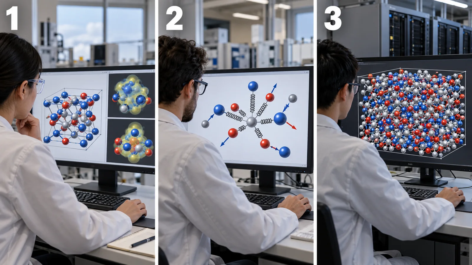
Original SVG reference: Concept diagram (vector drawing). How an MLIP is built and used. (1) Make training data with DFT, (2) train, (3) use in MD and so on, (4) check on systems not used in training. For regions that are missing, add data and retrain (active learning). The box below quotes what the papers say about speed.

Adding data for missing regions and retraining is called active learning. For MLIPs, methods that pick the training configurations automatically from the data have been studied, as in the paper by Podryabinkin and Shapeev (2017) Sourced[Ref. 7].

A common misconception: "An MLIP replaces first-principles calculation"

An MLIP is a model that imitates DFT. It inherits the errors of the teacher DFT (the approximation in the exchange-correlation functional and so on) as they are. On top of that, outside the range it learned it also departs from the DFT answer (the small experiment in chapter 7). An MLIP is useful in the sense of "speeding up everyday calculation so that DFT is used only where needed and as often as needed" (commentary).

3. How it works: from environment to per-atom energy, and then to forces

Most MLIPs use the following idea. Give each atom "an energy set by its surrounding environment", and add them all up to get the energy of the whole system. The M3GNet paper says: atomic energies come from the atomic information, and they sum to the total energy; the derivatives of the total energy give force and stress Sourced[Ref. 9].

Fig. 3. Conceptual illustration generated with ImageGen. A model may estimate local contributions and combine them into total energy. Not every potential uses exactly this architecture.Not an actual product, facility or measurement. Enlarged models, lines, arrows and colours are explanatory.

View original SVG, values and sources

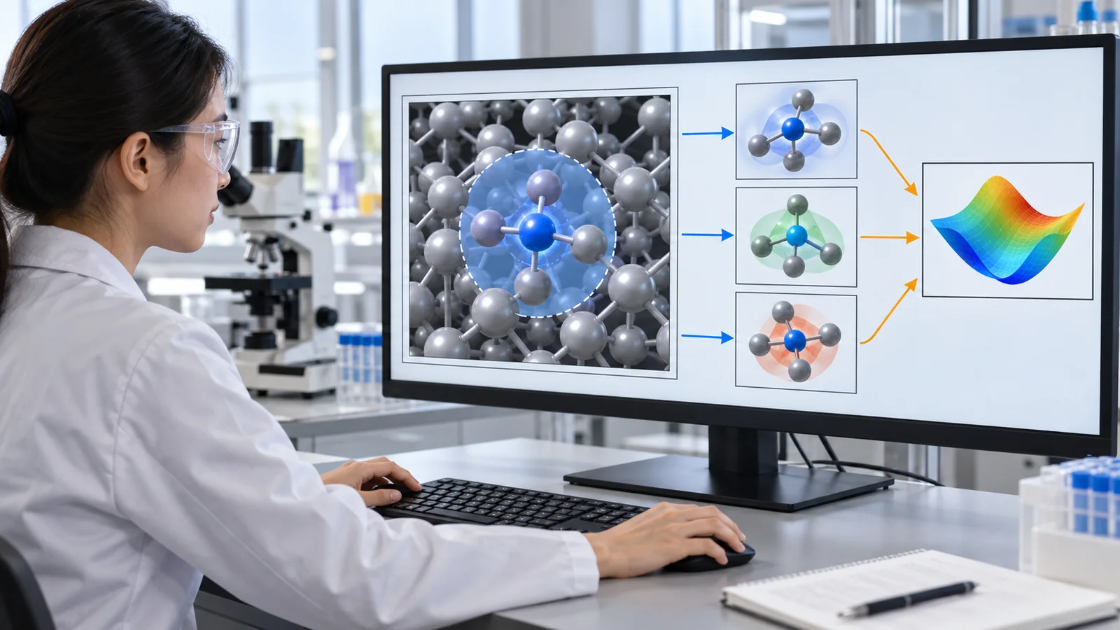
Original SVG reference: Concept diagram (vector drawing). Inside an MLIP. The environment (distances, angles, elements) of a focus atom within the cutoff radius r_cut is turned into numbers; the model returns an atomic energy ε; they are summed to the total energy E; and the forces come from its slope.

Turning the environment into numbers: some methods use hand-made numbers (descriptors), as in the method of Behler and Parrinello; others treat the arrangement of atoms as a graph (points and lines) and let a graph neural network make the numbers (see our explainer on graph neural networks)
Respecting natural symmetries: the energy does not change if you rotate the system, shift it, or swap atoms of the same element. The Deep Potential paper says the model preserves all the natural symmetries of the problem Sourced[Ref. 3]. NequIP uses an equivariant (E(3)-equivariant) network whose outputs change correctly under rotation and so on Sourced[Ref. 5]
The force is the slope of the energy: differentiate the model that outputs energy and you get the forces (the last step in Fig. 3). So training on forces as well as energy improves the force accuracy. In a table in the M3GNet paper, a model trained on energy only had a force error (MAE) of 379.4 meV/Å, against 70.2 meV/Å when trained on energy and forces Sourced[Ref. 9]
The "surrounding environment" has a range: atoms beyond the cutoff do not enter the energy of an atom. The MACE-MP-0 paper says two message-passing steps give an effective receptive field of about 12 Å, and warns that long-range interactions (electrostatics and so on) beyond it cannot be captured by a short-range model Sourced[Ref. 12]

Where people get stuck: "What does equivariant mean?"

Suppose you rotate a crystal in coordinate space. The material is the same, so the energy does not change (invariant). But a force is a quantity with a direction, so when the crystal is rotated, the force arrows must rotate with it (equivariant). The aim of equivariant models is that, if this property is built in from the start, learning is easier even with little data. The authors of the NequIP paper claim that high accuracy was obtained with little training data [Ref. 5] (commentary).

4. The main models and the universal (foundation) models

The ideas behind MLIPs have developed from the neural network of 2007, through Gaussian processes and deep networks, to equivariant graph neural networks. Since about 2022, "universal" or "foundation" models that handle a wide part of the periodic table with a single model have appeared one after another. Here we line up what we could confirm in papers and official pages. We do not rank them.

Fig. 4. Concept diagram (vector drawing). The main MLIPs in order of publication. Orange and red boxes are universal or foundation models; red marks preprints (not peer-reviewed). No ranking is implied, as evaluation conditions differ. Checked on 22 October 2026.

Model	Training data (as stated in the paper or official page)	Target and features	Evaluation conditions and reading notes
Behler-Parrinello (2007), GAP (2010)	DFT results (bulk silicon and others) [Refs. 1, 2] Sourced	Neural network / Gaussian process. GAP has no fixed functional form and can be improved systematically by adding data	Built separately for systems of limited scope. A different purpose from universal models
M3GNet (2022)	Materials Project structure-relaxation data: 187,687 ionic steps from 62,783 compounds, 89 elements. DFT: PBE / PBE+U. Split 90% / 5% / 5% by material, not by data point [Ref. 9] Sourced	A graph neural network with three-body interactions. Universal (periodic table)	On the test data, energy MAE 34.7±3.1 meV/atom, force 71.7±1.1 meV/Å, stress 0.41 GPa (model trained on energy, forces and stress) [Ref. 9] Sourced. The spread of the data (MAD) is 1345.6 meV/atom
CHGNet (2023)	MPtrj (about ten years of Materials Project DFT trajectories), 1,580,395 atomic configurations. Magnetic moments are also learned. GGA / GGA+U [Ref. 11] Sourced	A graph neural network including charge (magnetic-moment) information. Universal	On the MPtrj test data (14,572 materials, 157,955 structures): energy error 30 meV/atom, force 77 meV/Å, stress 0.348 GPa. Split 8:1:1 by compound [Ref. 11] Sourced
MACE (2022), MACE-MP-0 (2023)	MACE-MP-0: trained on MPtrj; 89 elements; DFT is PBE (+U) [Refs. 12, 13] Sourced	MACE: an equivariant model with higher-order many-body messages (preprint) [Ref. 6]. MACE-MP-0: a foundation model tried on solids, liquids, gases, interfaces and even a small protein	The authors say it can be used "qualitatively and at times quantitatively", and mention fine-tuning with a handful of data points. They state limits: short range only, no magnetic or spin degrees of freedom, and inconsistencies from the DFT settings in MP [Ref. 12] Sourced
MatterSim (2024, preprint)	Built by active learning from large-scale first-principles calculations (the authors) [Ref. 14] Sourced	A universal model across the periodic table, for 0 to 5000 K and up to 1000 GPa (the authors' claim)	"Up to ten-fold better precision than the prior best" and "Gibbs free energy up to 1000 K at a resolution of 15 meV/atom against experiment" are the authors' claims in a non-peer-reviewed preprint [Ref. 14]. The code license is shown as MIT [Ref. 15]
OMat24 (2024, preprint)	Data of over 110 million DFT calculations emphasising structural and compositional diversity, with pretrained models (EquiformerV2) [Ref. 16] Sourced	An inorganic-materials dataset and foundation models	The authors state state-of-the-art performance on the Matbench Discovery leaderboard, an F1 score above 0.9 and an energy accuracy of 20 meV/atom (the authors' claim, preprint). The data are CC-BY-4.0 [Ref. 17]; the models carry a separate OMat24 license
UMA (2025, preprint)	About half a billion atomic structures, combining data from several domains such as molecules, materials and catalysts [Ref. 18] Sourced	"Universal Models for Atoms". The authors say they perform similarly to or better than specialised models	The authors' claim, preprint. The models are released under the FAIR Chemistry License v1 and an Acceptable Use Policy [Ref. 19]

The accuracy figures of the models cannot be set side by side, because the way the data were split, the data used for evaluation and the DFT settings differ. A preprint is a description that has not passed peer review.

Fig. 5. Diagram including our calculation (vector drawing). The scale of the training data on a logarithmic axis (as stated in the papers). The unit counted differs slightly.

A common misconception: "The more training data, the more accurate it is, always"

It is not only the amount of data; quality, bias and the way the data are split matter. For example, Deng et al. (2025) report that M3GNet, CHGNet and MACE-MP-0 all give energies and forces that are systematically too small (the potential energy surface is "too soft"), and trace this to the pretraining data being biased toward near-equilibrium atomic arrangements Sourced[Refs. 25, 26]. More data may not remove this kind of error if the bias remains (commentary).

5. What "near first-principles accuracy" and "orders of magnitude faster" mean

The slogan of MLIPs is "first-principles accuracy, orders of magnitude faster". Let us check the two halves against what the papers say.

Speed: Behler and Parrinello (2007) say it is several orders of magnitude faster than DFT (bulk silicon) Sourced[Ref. 1]. Bartók et al. (2010) say it saves orders of magnitude in computational cost when generating long MD trajectories Sourced[Ref. 2]. Zhang et al. (2018) say the cost scales linearly with system size Sourced[Ref. 3]. Jia et al. (2020) report MD of more than 100 million atoms at more than 1 ns per day with a dedicated code on the Summit supercomputer Sourced[Ref. 4]. But these are values for particular systems and machines, not a factor you can count on every time
Accuracy: "near first-principles" means how close the result is to the DFT result used as the teacher. It does not mean agreement with measurement. The M3GNet paper says that the phonon results come out systematically lower than DFT, and that this is "likely" due to the different functionals of the training data (PBE / PBE+U) and of the DFT phonon calculation compared against (PBEsol) Sourced[Ref. 9]. The DFT settings of the teacher influence the character of the prediction

A materials engineer's view 1: read MLIP accuracy in two stages: "the teacher's DFT settings" and "the gap to measurement"

Stage one is how well the MLIP reproduces DFT (the error tables). Stage two is how well the DFT itself reproduces measurement. For example, the MACE-MP-0 paper says that the Materials Project DFT (PBE without a Hubbard U) cannot tell Ce³⁺ from Ce⁴⁺ in ceria nanoparticles, and neither could MACE-MP-0 Sourced[Ref. 12]. An MLIP cannot newly create a distinction its teacher does not have. For a property that DFT is known to get wrong for your material, assume the MLIP will get it wrong too (commentary).

6. How to read accuracy numbers

MLIP papers carry numbers such as "energy error 30 meV/atom". How should we read them? As a materials engineer, check three points.

Fig. 6. Diagram including our calculation (vector drawing). MLIP energy errors (MAE) set beside the thermal energy at room temperature and the scale of crystal stability. The CHGNet and M3GNet values come from the test data in each paper (arXiv versions) and are not a comparison on the same data.

An average of what (MAE): the MAE (mean absolute error) is the average of the absolute errors. Large errors at outliers are buried. The CHGNet energy error of 30 meV/atom and the M3GNet error of 34.7 meV/atom are about 1.2 to 1.3 times the thermal energy at room temperature (300 K), k_B T = 25.9 meV Our calculation. Crystal stability is judged by "the height of the energy above the convex hull", and the M3GNet paper quotes that 90% of the crystals in the ICSD lie less than 67 meV/atom above the hull Sourced[Ref. 9]. The error is about as large as the scale used for the judgement
On which data: both numbers are for test data split from the same Materials Project as the training data (M3GNet split by material, CHGNet by compound) [Refs. 9, 11]. The error for new compositions or structures can be larger. To address this, Matbench Discovery uses 257,487 structures made by a different route (WBM) for testing, and removes structures that overlap with the training data (MP) Sourced[Ref. 21]
Does a small error suffice for the purpose: the Matbench Discovery paper points out that regression metrics (error) and classification metrics for judging stability do not line up: even an accurate regressor can produce more wrong calls near the decision boundary (on the hull) Sourced[Ref. 21]. Fu et al. (2023) show that even with small force errors, this is a different matter from the quantities that count in MD (for example, whether it runs stably), and name stability as an important metric Sourced[Ref. 23]

Where people get stuck: "MAE", "MAD" and "convex hull"

MAE is "the average difference between prediction and truth", and MAD is "the average spread of the data itself". Comparing MAE with MAD shows the relative size of the error (about 2.6% for M3GNet) Our calculation. The convex hull is the line joining the lowest-energy combinations of phases at a given composition; the higher a material sits above it, the more likely it is to decompose (see our explainer on crystal structure prediction and stability). If the error is as large as "how far above the hull", the call of stable versus unstable becomes unreliable.

7. Cautions in use: outside the learned range

Machine learning was "an approximator that learns trends from past data". It is weak outside the range of the data (extrapolation). The same happens with MLIPs. First, here is a drastically simplified example.

Fig. 7. Diagram including our calculation (vector drawing). A small experiment in which a Gaussian process learns the energy of two atoms (Lennard-Jones type). The green band is the range used for training (10 points). Inside it the curve is reproduced almost perfectly, but on the side where the atoms are too close (the wall) it goes far off.

Inside the range: the largest error was 0.009 (about 1% of the well depth ε = 1) Our calculation
Outside the range (too close): at r = 0.95σ the prediction was −0.27 against a true value of 1.96. The model has not learned that a "wall" rises there Our calculation
The model's own uncertainty (σ): the uncertainty it reported was 0.33, and the actual error of 2.23 was about 7 times that Our calculation. Even uncertainty estimates can be unreliable outside the range
Adding one data point: adding a single point at r = 0.98 brought the prediction at r = 0.95 to 1.32 Our calculation. But this is a small example, not a direct picture of how a real MLIP behaves

Problems of the same kind have been reported for real MLIPs.

Systematic softening: Deng et al. (2025) report that three universal MLIPs, M3GNet, CHGNet and MACE-MP-0, consistently under-predict energy and force in tasks such as surfaces, defects, solid solutions, phonons, ion-migration barriers and high-energy states. They attribute it to an under-estimated curvature of the potential energy surface, arising from pretraining data biased toward near-equilibrium configurations. And they show that it can be largely corrected by fine-tuning with one additional data point Sourced[Refs. 25, 26]
Good energy and force do not guarantee properties: Loew et al. (2025) evaluated universal MLIPs on about 10,000 first-principles phonon calculations. They report that some models that predict energy and force well for materials near equilibrium are substantially inaccurate for harmonic phonons Sourced[Ref. 24]
Limits the authors themselves state: the MACE-MP-0 paper says that a short-range model can leave some observables uncomputable, especially for dilute solutions and interfaces, and that it has no magnetic or spin degrees of freedom Sourced[Ref. 12]

A common misconception: "A model with high accuracy will be right on unseen materials too"

The meaning of an accuracy number depends on which data it was measured on. If the test data come from the same distribution as the training data, the accuracy on new materials can be lower. The Matbench Discovery paper tries to address this by using test data made by a different route (WBM) and removing structures that overlap with the training data (MP) Sourced[Ref. 21]. Even so, the accuracy for materials beyond the range used in the evaluation (your additives, interfaces and so on) has to be checked by yourself (commentary).

8. How to use one: as is, fine-tuned, or dedicated

Fig. 8 summarises the flow for using a universal model in real work. The key is three checks: is the target inside the range of the training data, do your own simple quantities agree with DFT or measurement, and is uncertainty watched in production runs.

Fig. 8. Concept diagram (vector drawing). The flow of checks when using a universal MLIP. If the answer to Q1 to Q3 is "no", deal with it by training a dedicated model, fine-tuning, or monitoring uncertainty.

Fine-tuning: the MACE-MP-0 paper says a foundation model can be fine-tuned on a handful of application-specific data points to reach near-DFT accuracy Sourced[Ref. 12]. Deng et al. (2025) also report that one added point can correct the systematic softening [Ref. 25]
Check the licenses: the code, the pretrained weights and the training data may carry separate licenses. For example, the MACE code is published under the MIT License [Ref. 27] and the CHGNet code under a BSD-style license [Ref. 28]. The MACE-MP-0 family of models is listed as MIT, and MACE-OMAT-0 and others as "ASL" (we could not confirm what the abbreviation stands for) [Ref. 13]. The OMat24 data are CC-BY-4.0 [Ref. 17], and UMA comes with the FAIR Chemistry License v1 and an acceptable-use policy [Ref. 19] Sourced. Check the license text to see whether commercial use is allowed (this article is not legal advice)
Software changes fast: when we checked on 22 October 2026, the official MACE-foundations repository listed, besides the MP-0 family, models of several generations, several training datasets and several DFT settings (PBE+U, PBE, r²SCAN and so on). The same name may mean different behaviour in different versions, so record the version and the date Sourced[Ref. 13]

9. A materials engineer's view

A materials engineer's view 2: check first whether your material is inside the "range of the training data"

The training data of M3GNet, CHGNet and MACE-MP-0 are centred on calculations of inorganic crystals in the Materials Project [Refs. 9, 11, 12]. Polymers, solutions, interfaces, amorphous materials, systems with dopants and strongly correlated electron systems may not be well represented (inference; we have not checked the content individually). First confirm, in the model's paper or official page, "whether the elemental combination, structure, temperature and pressure of your material are in the training data". If not, go to a dedicated model or back to first principles, as in Fig. 8.

A materials engineer's view 3: decide your own "simple acceptance test" before adoption

Before using a universal model, check three quantities on your own material. (1) The energy-versus-volume curve (compress and stretch the crystal by a few percent and compare with DFT; this is a tell-tale of "systematic softening"). (2) The lattice constant, elastic modulus and thermal expansion, whichever you have measurements for. (3) Phonons (vibration frequencies). Phonons can go wrong even when energy and force accuracy is high [Ref. 24]. Do not use a model for that material if it disagrees with DFT or measurement on these three (commentary).

Fig. 9. Conceptual illustration generated with ImageGen. Check forces and application-relevant behaviour, not only energy, against independent references. Record the model and data domain.Not an actual product, facility or measurement. Enlarged models, lines, arrows and colours are explanatory.

A materials engineer's view 4: keep your own calculation and experiment data in a form that can be used for training

The quality of an MLIP is decided by data. For your own DFT calculations, keep the functional, the software and its version, the cutoff, the k-points and the history of the structure. For experimental data, attach the sample's manufacturing route, thermal history, measurement conditions and lot. Keep calculations that did not converge and experiments that did not work as failure data too. They are valuable for finding the regions where a model is weak and for choosing the points for fine-tuning.

10. Limits, what we could not confirm, and a summary

Summary of this article

An MLIP is an approximator that learns "atomic arrangement → energy and forces" from DFT results. It adds per-atom energies to get the total energy, and gets the forces from its slope Sourced
Universal (foundation) models target a wide part of the periodic table, but they have limits in the range of training data (mostly from the Materials Project), the DFT settings, the short-range assumption and so on. Which is better cannot be asserted because conditions differ Sourced
Read accuracy numbers together with the error metric, the evaluation data and the way of splitting. An energy error of 30 meV/atom is about 1.2 times the thermal energy at room temperature, comparable to the scale used to judge stability Our calculation
It goes wrong outside the learned range. In our small experiment the largest error was 0.009 inside the range and 2.23 outside it. Systematic softening and phonon errors have also been reported for real universal models Our calculationSourced

What we could not confirm

We did not reproduce every number in each model's paper back to the original data. This article organises the statements and tables of the papers (arXiv versions included). The numbers for CHGNet, M3GNet and Matbench Discovery come from the arXiv versions, and we did not check differences from the published versions
MatterSim, OMat24 and UMA are described as of their preprints (at the checking date), and we did not check any post-review versions. Accuracy claims are written as the authors' claims
We could not confirm what the license abbreviation "ASL" (MACE-OMAT-0 and others) stands for, or its conditions
We did not check individually how many systems (polymers, interfaces, amorphous materials and so on) the training data of universal models contain
The cost of DFT (how it grows with the number of atoms) is covered in other articles, so we give no figures here
We could not find an international standard specific to MLIPs

11. How to read the yardsticks and standards

The yardsticks for MLIPs are first how well it reproduces the teacher DFT (errors in energy, force and stress), then whether predictions for new materials and conditions are right (stability classification, structure optimisation, phonons, stability of MD), and then whether it reproduces measurement. What the yardsticks do not measure is the range outside what was learned and the error of the teacher DFT itself. Checked on 22 October 2026.

Item	Representative benchmarks and methods (name, source)	Standards and guidance (ISO/IEC, NIST, CEN, etc.)	Reading notes
Errors (energy, force, stress)	MAE on the test data of each paper. M3GNet: energy 34.7 meV/atom, force 71.7 meV/Å, stress 0.41 GPa [Ref. 9]. CHGNet: 30 meV/atom, 77 meV/Å, 0.348 GPa [Ref. 11] Sourced	Could not be confirmed	The split (by material / by compound) and the data (MP test sets) differ. Not a comparison on the same footing
Stability classification (searching for new materials)	Matbench Discovery (Riebesell et al.): training on MP, testing on 257,487 WBM structures. Evaluated with F1, DAF (discovery acceleration factor) and so on [Refs. 20, 21] Sourced	Could not be confirmed	In the initial results, regression and classification metrics did not line up. The leaderboard keeps being updated. Models with different training data are hard to compare on the same footing
The leaderboard today	The official site has tasks beyond stability classification (geometry optimisation, MD, phonons, diatomics) and shows a combined score CPS (discovery F1 50%, geometry RMSD 10%, phonon κ SRME 40%) (checked 22 October 2026) [Ref. 22] Sourced	Could not be confirmed	The weights of the metrics follow the site's design. A rank is not the same as how well a model performs on your material
Stability of MD and evaluation close to real use	Fu et al. (2023): force errors do not line up with the quantities that matter in MD; stability matters [Ref. 23] Sourced	Could not be confirmed	Small force errors alone do not guarantee that MD runs stably
Properties (phonons and so on)	Loew et al. (2025): evaluation on about 10,000 first-principles phonon calculations [Ref. 24] Sourced	Could not be confirmed	Some models with good energy and force are off on phonons
Outside the learned range and systematic errors	Deng et al. (2025): systematic softening in three universal models [Ref. 25] Sourced	Could not be confirmed	Errors from data bias, unlike random errors, can sometimes be corrected
Public repositories and records	The NIST Interatomic Potentials Repository [Ref. 29]; OpenKIM, a curated repository of interatomic potentials including machine-learning ones [Ref. 30] Sourced	CEN CWA 17284:2018: terminology and a documentation template (MODA) for materials modelling. It states that it covers physics-based models and not data-based models; a MODA for data-based models is said to be in a separate document (RoMM) [Ref. 31] Sourced. Not an official standard	An MLIP is a data-based model, so it is outside the direct scope of the CWA
Frameworks for AI in general	NIST AI Risk Management Framework 1.0 (released 26 January 2023): a voluntary framework. NIST's page notes that revision is under way (at the checking date) [Ref. 32] SourcedNot yet confirmed	We could not find an international standard specific to MLIPs	General AI guidance does not go as far as how to read MLIP errors

The organisation of the table is Our calculation (our arrangement). Numbers, titles and values were checked in papers and on official pages (checked on 22 October 2026). The standards are all recommendations, terminology or voluntary frameworks, not standards with legal force. We did not confirm any applicable ASTM standard within the scope of this article.

Reading notes (for materials engineers)

Being near the top of a leaderboard does not mean it will be right for your material: a rank is an evaluation on set tasks and data. Test your own material with simple acceptance tests
Keep prediction apart from experimental confirmation: that an MLIP calls a material "stable" does not mean it can be made or has the properties; that needs separate confirmation (see our explainer on crystal structure prediction and stability)
Data leakage and split pitfalls: if the test data are close to the training data, accuracy looks high. Matbench Discovery removes overlapping structures [Ref. 21]. When reading a paper, check how the data were split
Are standards and guidance recommended or required? The guidance cited here (NIST AI RMF and so on) is a voluntary framework, and the CWA is not an official standard [Refs. 32, 31]
Model version and date: the same name can mean different behaviour across generations. Record the version you used [Ref. 13]

12. Glossary

Machine-learning interatomic potential (MLIP): An approximator that returns energy and forces from an arrangement of atoms.

First-principles calculation / DFT: A physics simulation that computes the energy of matter from the behaviour of electrons. Density functional theory. Contains approximations.

Potential energy surface: The relation between atomic arrangement and energy. Its slope gives the force.

Training data: The pairs of "arrangement and energy / forces" the model learns. For MLIPs, DFT results.

Descriptor: A "business card" of a material in numbers. Here, the environment (distances, angles) turned into numbers.

Graph neural network (GNN): A neural network that handles a graph with atoms as points and bonds as lines.

Equivariant (E(3)-equivariant): The property that outputs such as forces rotate in the same way when the system is rotated.

Cutoff: The range (radius) of surrounding atoms that enter an atom's energy.

Universal MLIP / foundation model: A model that tries to handle a wide part of the periodic table with one model.

Fine-tuning: Adjusting a trained model with a small amount of additional data.

Active learning: A method in which the model picks and adds data for missing regions and retrains.

MAE / MAD: Mean absolute error / mean absolute deviation of the data itself. Used to see the relative size of the error.

Convex hull (energy above hull): The line joining the lowest-energy phase combinations at a composition. The height above it is a rough measure of instability.

MP / MPtrj: Materials Project (a computed database of inorganic materials) / its DFT trajectory dataset (assembled in the CHGNet paper).

PBE / PBE+U: A kind of exchange-correlation functional in DFT / the same with a correction U for electron localisation.

Extrapolation: Prediction outside the range of the data learned. Prone to errors.

Systematic softening: The tendency for energy and force to come out consistently too small (reported by Deng et al.).

Phonon: A vibrational mode of the atoms in a crystal. Linked to heat conduction and stability.

F1 / DAF: A classification metric / the discovery acceleration factor (Matbench Discovery).

License: The terms of use for code, weights and data. They can differ from one to the next.

Preprint: A paper made public before peer review, for example on arXiv.

13. References

Behler J., Parrinello M. "Generalized Neural-Network Representation of High-Dimensional Potential-Energy Surfaces", Phys. Rev. Lett. 98, 146401 (2007), DOI 10.1103/PhysRevLett.98.146401 — doi.org/10.1103/PhysRevLett.98.146401
Bartók A. P., Payne M. C., Kondor R., Csányi G. "Gaussian Approximation Potentials: The Accuracy of Quantum Mechanics, without the Electrons", Phys. Rev. Lett. 104, 136403 (2010), DOI 10.1103/PhysRevLett.104.136403 — doi.org/10.1103/PhysRevLett.104.136403
Zhang L., Han J., Wang H., Car R., E W. "Deep Potential Molecular Dynamics: A Scalable Model with the Accuracy of Quantum Mechanics", Phys. Rev. Lett. 120, 143001 (2018), DOI 10.1103/PhysRevLett.120.143001 — doi.org/10.1103/PhysRevLett.120.143001
Jia W. et al. "Pushing the limit of molecular dynamics with ab initio accuracy to 100 million atoms with machine learning", arXiv:2005.00223 (SC20) (2020) — arxiv.org/abs/2005.00223
Batzner S. et al. "E(3)-equivariant graph neural networks for data-efficient and accurate interatomic potentials", Nat. Commun. 13, 2453 (2022), DOI 10.1038/s41467-022-29939-5 — doi.org/10.1038/s41467-022-29939-5
Batatia I. et al. "MACE: Higher Order Equivariant Message Passing Neural Networks for Fast and Accurate Force Fields", arXiv:2206.07697 (preprint) (2022) — arxiv.org/abs/2206.07697
Podryabinkin E. V., Shapeev A. V. "Active learning of linearly parametrized interatomic potentials", Comput. Mater. Sci. 140, 171–180 (2017), DOI 10.1016/j.commatsci.2017.08.031 — doi.org/10.1016/j.commatsci.2017.08.031
Chen C., Ong S. P. "A universal graph deep learning interatomic potential for the periodic table", Nat. Comput. Sci. 2, 718–728 (2022), DOI 10.1038/s43588-022-00349-3 — doi.org/10.1038/s43588-022-00349-3
Chen C., Ong S. P. A universal graph deep learning interatomic potential for the periodic table (arXiv version, the numbers in this article are taken from it), arXiv:2202.02450 (2022) — arxiv.org/abs/2202.02450
Deng B. et al. "CHGNet as a pretrained universal neural network potential for charge-informed atomistic modelling", Nat. Mach. Intell. 5, 1031–1041 (2023), DOI 10.1038/s42256-023-00716-3 — doi.org/10.1038/s42256-023-00716-3
Deng B. et al. CHGNet: Pretrained universal neural network potential for charge-informed atomistic modeling (arXiv version, the numbers in this article are taken from it), arXiv:2302.14231 (2023) — arxiv.org/abs/2302.14231
Batatia I. et al. "A foundation model for atomistic materials chemistry", arXiv:2401.00096 (v3, preprint) (2023) — arxiv.org/abs/2401.00096
ACEsuit "MACE-foundations repository README (model list with training dataset, level of theory and license columns)" — github.com/ACEsuit/mace-foundations
Yang H. et al. "MatterSim: A Deep Learning Atomistic Model Across Elements, Temperatures and Pressures", arXiv:2405.04967 (preprint) (2024) — arxiv.org/abs/2405.04967
Microsoft "mattersim repository (license shown by GitHub: MIT)" — github.com/microsoft/mattersim
Barroso-Luque L. et al. "Open Materials 2024 (OMat24) Inorganic Materials Dataset and Models", arXiv:2410.12771 (preprint) (2024) — arxiv.org/abs/2410.12771
Hugging Face (facebook) "OMAT24 dataset card (license: cc-by-4.0)" — huggingface.co/datasets/facebook/OMAT24
Wood B. M. et al. "UMA: A Family of Universal Models for Atoms", arXiv:2506.23971 (preprint) (2025) — arxiv.org/abs/2506.23971
Hugging Face (facebook) "UMA model page (FAIR Chemistry License v1, Acceptable Use Policy)" — huggingface.co/facebook/UMA
Riebesell J. et al. "A framework to evaluate machine learning crystal stability predictions", Nat. Mach. Intell. 7, 836–847 (2025), DOI 10.1038/s42256-025-01055-1 — doi.org/10.1038/s42256-025-01055-1
Riebesell J. et al. Matbench Discovery - A framework to evaluate machine learning crystal stability predictions (arXiv version, the numbers in this article are taken from it), arXiv:2308.14920 (2023) — arxiv.org/abs/2308.14920
Matbench Discovery "Leaderboard website (checked 22 October 2026)" — matbench-discovery.materialsproject.org/
Fu X. et al. "Forces are not Enough: Benchmark and Critical Evaluation for Machine Learning Force Fields with Molecular Simulations", Transactions on Machine Learning Research (arXiv:2210.07237) (2023) — arxiv.org/abs/2210.07237
Loew A. et al. "Universal machine learning interatomic potentials are ready for phonons", npj Comput. Mater. 11, 178 (2025), DOI 10.1038/s41524-025-01650-1 — doi.org/10.1038/s41524-025-01650-1
Deng B. et al. "Systematic softening in universal machine learning interatomic potentials", npj Comput. Mater. 11, 9 (2025), DOI 10.1038/s41524-024-01500-6 — doi.org/10.1038/s41524-024-01500-6
Deng B. et al. Overcoming systematic softening in universal machine learning interatomic potentials by fine-tuning (arXiv version, the abstract is cited), arXiv:2405.07105 (2024) — arxiv.org/abs/2405.07105
ACEsuit "mace repository, LICENSE.md (MIT License)" — github.com/ACEsuit/mace/blob/main/LICENSE.md
CederGroupHub "chgnet repository, LICENSE (BSD-style license of the University of California and Lawrence Berkeley National Laboratory)" — github.com/CederGroupHub/chgnet/blob/main/LICENSE
NIST (National Institute of Standards and Technology) "Interatomic Potentials Repository" — www.ctcms.nist.gov/potentials/
OpenKIM "Knowledgebase of Interatomic Models (OpenKIM)" — openkim.org/
CEN (European Committee for Standardization) "CEN Workshop Agreement CWA 17284:2018, Materials modelling - Terminology, classification and metadata" (2018) — www.cencenelec.eu/media/CEN-CENELEC/CWAs/RI/cwa17284_2018.pdf
NIST (National Institute of Standards and Technology) "AI Risk Management Framework (AI RMF 1.0, released 26 January 2023; page checked 22 October 2026)" — www.nist.gov/itl/ai-risk-management-framework

14. Claim-to-source audit

Claim in the text	Basis	Type
The idea of MLIPs: build a neural network that returns energy and forces from DFT results. DFT is unsuited to long calculations of large systems. Behler and Parrinello (2007): several orders of magnitude faster than DFT (demonstrated on bulk silicon)	Reference 1 https://doi.org/10.1103/PhysRevLett.98.146401	Sourced
Bartók et al. (2010): Gaussian approximation potentials have no fixed functional form, are generated automatically from data and can be improved systematically with more data. They save orders of magnitude in the cost of long MD trajectories	Reference 2 https://doi.org/10.1103/PhysRevLett.104.136403	Sourced
Zhang et al. (2018): Deep Potential is a many-body potential built with a deep network, preserves natural symmetries, and its cost is linear in system size. Jia et al. (2020): over 100 million atoms, more than 1 ns per day (Summit, dedicated code)	Reference 3 https://doi.org/10.1103/PhysRevLett.120.143001 Reference 4 https://arxiv.org/abs/2005.00223	Sourced
CHGNet paper: classical force fields often fail to describe the coupling between electronic states and ionic rearrangements. CHGNet is pretrained on MPtrj (about ten years, about 1.5 million structures) and also learns magnetic moments	Reference 11 https://arxiv.org/abs/2302.14231	Sourced
How M3GNet works: atomic energies are summed to the total energy, and its derivatives give force and stress. Training data (MPF.2021.2.8): 187,687 steps, 62,783 compounds, 89 elements, split 90% / 5% / 5% by material	Reference 9 https://arxiv.org/abs/2202.02450	Sourced
M3GNet error table: force MAE 379.4 meV/Å for the model trained on energy only, 70.2 for energy and forces, 71.7 for energy, forces and stress. MAE of the energy-force-stress model: energy 34.7±3.1 meV/atom, stress 0.41 GPa. Spread of the data (MAD): energy 1345.6 meV/atom	Reference 9 https://arxiv.org/abs/2202.02450	Sourced
M3GNet: 90% of the inorganic crystals in the ICSD lie less than 0.067 eV/atom above the hull (a value quoted in the paper). The systematically low phonons are likely due to the difference between the functional of the training data (PBE / PBE+U) and that of the comparison data (PBEsol)	Reference 9 https://arxiv.org/abs/2202.02450	Sourced
M3GNet (Nat. Comput. Sci. 2022): a universal interatomic potential. A graph neural network with three-body interactions. Trained on Materials Project structure-relaxation data	Reference 8 https://doi.org/10.1038/s43588-022-00349-3	Sourced
CHGNet on its test data (14,572 materials, 157,955 structures): MAE of energy 30 meV/atom, force 77 meV/Å, stress 0.348 GPa (with magnetic moments). MPtrj has 1,580,395 atomic configurations. Split 8:1:1 by compound	Reference 11 https://arxiv.org/abs/2302.14231	Sourced
CHGNet (Nat. Mach. Intell. 2023): a pretrained universal neural-network potential including charge information	Reference 10 https://doi.org/10.1038/s42256-023-00716-3	Sourced
MACE: an equivariant model with higher-order many-body messages (preprint). NequIP: an E(3)-equivariant graph neural network; the authors claim high accuracy from little training data	Reference 6 https://arxiv.org/abs/2206.07697 Reference 5 https://doi.org/10.1038/s41467-022-29939-5	Sourced
MACE-MP-0: a universal foundation model trained on MPtrj. Applied to solids, liquids, gases, interfaces and a small protein. Can be fine-tuned with a handful of data. Limits: short range only (about 12 Å), no magnetic or spin degrees of freedom, constraints from PBE (+U) in MP. Cannot tell Ce³⁺ from Ce⁴⁺ in ceria nanoparticles	Reference 12 https://arxiv.org/abs/2401.00096	Sourced
Official README of MACE-foundations (checked 22 October 2026): MP-0 family, MPA-0, OMAT-0, MATPES, OMOL, MH and other models. 89 elements. DFT settings: PBE+U, PBE, r²SCAN and so on. License column: MIT for the MP-0 family, ASL for OMAT-0 and others	Reference 13 https://github.com/ACEsuit/mace-foundations	Sourced
MatterSim (preprint): built by active learning from large-scale first-principles calculations. 0 to 5000 K, up to 1000 GPa. "Up to ten-fold better precision than the prior best" and "Gibbs free energy up to 1000 K at 15 meV/atom against experiment" are the authors' claims. Code under MIT	Reference 14 https://arxiv.org/abs/2405.04967 Reference 15 https://github.com/microsoft/mattersim	Sourced
OMat24 (preprint): over 110 million DFT calculations. EquiformerV2 models. State of the art on Matbench Discovery, F1 above 0.9 and 20 meV/atom are the authors' claims. Data under CC-BY-4.0	Reference 16 https://arxiv.org/abs/2410.12771 Reference 17 https://huggingface.co/datasets/facebook/OMAT24	Sourced
UMA (preprint): trained on about half a billion atomic structures across several domains such as molecules, materials and catalysts. The authors claim that one model matches or beats specialised models. FAIR Chemistry License v1 and an acceptable-use policy	Reference 18 https://arxiv.org/abs/2506.23971 Reference 19 https://huggingface.co/facebook/UMA	Sourced
Deng et al.: systematic softening common to M3GNet, CHGNet and MACE-MP-0 (under-prediction for surfaces, defects, solid solutions, phonons, ion-migration barriers and high-energy states). Cause: pretraining data biased toward near-equilibrium. Corrected by one added point	Reference 25 https://doi.org/10.1038/s41524-024-01500-6 Reference 26 https://arxiv.org/abs/2405.07105	Sourced
Loew et al.: universal MLIPs evaluated on about 10,000 first-principles phonon calculations. Some models with good energy and force are badly off on phonons	Reference 24 https://doi.org/10.1038/s41524-025-01650-1	Sourced
Matbench Discovery: training on the Materials Project, testing on 257,487 WBM structures. Structures overlapping with MP are removed (11,175 materials). Regression and classification metrics do not line up. In the initial results the F1 of universal interatomic potentials was 0.57 to 0.82 and the discovery acceleration up to about 6 times	Reference 20 https://doi.org/10.1038/s42256-025-01055-1 Reference 21 https://arxiv.org/abs/2308.14920	Sourced
Matbench Discovery website (checked 22 October 2026): tasks beyond stability classification (geometry optimisation, MD, phonons, diatomics). Combined score CPS (F1 50%, RMSD 10%, κ SRME 40%). Many models (43 of 53 shown)	Reference 22 https://matbench-discovery.materialsproject.org/	Sourced
Fu et al.: force and energy errors do not line up with the quantities that matter in MD. Stability is an important metric	Reference 23 https://arxiv.org/abs/2210.07237	Sourced
Podryabinkin and Shapeev: active learning of linearly parametrized interatomic potentials	Reference 7 https://doi.org/10.1016/j.commatsci.2017.08.031	Sourced
Licenses: the MACE code is MIT; the CHGNet code is under a BSD-style license of the University of California and Lawrence Berkeley National Laboratory. Code, weights and data may carry separate licenses (this article is not legal advice)	Reference 27 https://github.com/ACEsuit/mace/blob/main/LICENSE.md Reference 28 https://github.com/CederGroupHub/chgnet/blob/main/LICENSE	Sourced
The NIST Interatomic Potentials Repository (with evaluation tools); OpenKIM (a curated public repository including machine-learning potentials)	Reference 29 https://www.ctcms.nist.gov/potentials/ Reference 30 https://openkim.org/	Sourced
CEN CWA 17284:2018: it covers physics-based models and excludes data-based models. A MODA for data-based models is in RoMM. Not an official standard	Reference 31 https://www.cencenelec.eu/media/CEN-CENELEC/CWAs/RI/cwa17284_2018.pdf	Sourced
NIST AI RMF 1.0: released 26 January 2023, voluntary. The page notes that revision is under way (at the checking date)	Reference 32 https://www.nist.gov/itl/ai-risk-management-framework	SourcedNot yet confirmed
k_B T at 300 K = 25.9 meV. The MAEs of CHGNet and M3GNet are about 1.2 to 1.3 times that. The MAE of 34.7 for M3GNet is about 2.6% of the MAD of 1345.6 (computed here from the formulas)	our calculation	Our calculation
Numbers of Fig. 7 (the small Gaussian-process experiment): largest error inside the range 0.009 (mean 0.0016); at r = 0.95σ true value 1.96, prediction −0.27, model uncertainty 0.33 (the error of 2.23 is about 7 times larger); prediction 1.32 after adding one point; mean error over 0.92-1.08 falls from 1.14 to 0.39	our calculation (Gaussian-process regression)	Our calculation
A materials engineer's views (the DFT settings of the teacher, the range of training data, acceptance tests before adoption, organising data). That polymers, interfaces and so on may not be well represented is an inference	commentary (our own view)
We could not find an international standard specific to MLIPs, nor the full name and terms of the ASL license	our own check (could not be confirmed)

Last updated: 22 October 2026. Sources are limited to primary material (papers, preprints, official GitHub, Hugging Face and Matbench Discovery pages, and documents from CEN and NIST). Numerical examples are our own calculations and do not directly show how a real MLIP behaves. We could not confirm reproduction of every number of each model against the original data, differences from published versions, the post-review content of the preprints, what the license abbreviation ASL stands for, the breakdown of systems in the training data of universal models, or any international standard specific to MLIPs, so we do not assert them. Figs. 2 to 8 are illustrative concept diagrams or drawings that include our calculations; Figs. 1 and 9 are AI-generated images (only the scene to be drawn is specified).