TECHNOLOGY EXPLAINER
Quantum Chemistry and Materials Simulation
What it means to compute the quantum behaviour of electrons on a quantum computer
Catalysts, batteries, magnets, superconductors: the properties of matter are set by the quantum behaviour of electrons. But as electrons are added, the number of values needed to compute this exactly explodes, and classical computers cannot cope. Quantum computers have long been expected to suit this task. This article uses figures and small numbers to show why it is hard, then explains how a calculation runs on a quantum computer (phase estimation, VQE and sample-based methods). It then sorts out, without exaggeration and from a materials engineer's viewpoint, the size and accuracy of molecules tried on real devices, the estimated scale needed, and the comparison with the best classical methods.
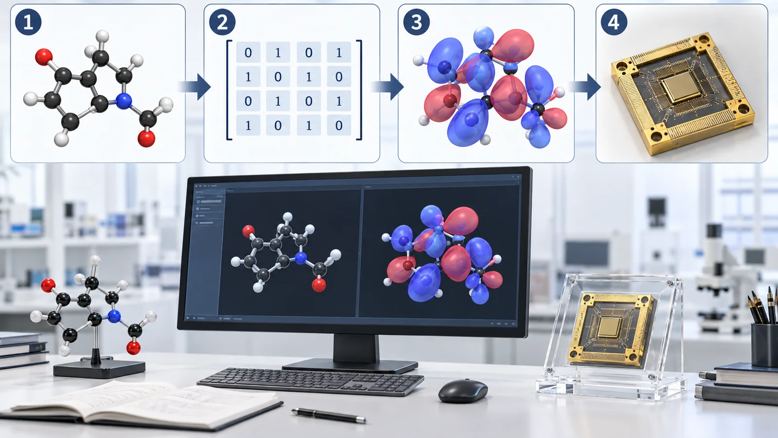
- The short version, what to know first, and where this fits in the series
- Why compute molecules and materials on a quantum computer?
- The quantum nature of electrons: why the numbers explode
- Classical methods: what they cover and where they struggle
- How a calculation runs on a quantum computer
- Molecules tried on real devices: scale and accuracy, without exaggeration
- Estimated scale needed: falling year by year, but still the future
- Comparison with classical methods: opinions are divided
- Materials simulation: lattice models and how they differ from molecules
- A materials engineer's view
- Limits, what we could not confirm, and a summary
- How to read evaluations and standards
- Glossary
- References
- Claim-to-source audit
Sourced = stated in a published source (linked)
Our calculation = a value computed in this article from the stated assumptions
Not yet confirmed = plans, targets, drafts, work in progress, outlooks: not settled
Our own reading for materials engineers is marked as commentary. Inference is shown in bold. Company announcements are labelled as company claims.
1. The short version, what to know first, and where this fits in the series
- The properties of molecules and materials are set by the behaviour of electrons (quantum mechanics). As electrons are added, the number of values needed for an exact calculation grows combinatorially, and about 22 electrons in 22 orbitals is considered the limit for classical computers. Since Feynman (1982) there has been the expectation that "quantum systems call for quantum computers" Sourced[Refs. 1, 17]
- The molecules tried on real devices are small, mostly of a size classical methods solve accurately. Even the largest example (77 qubits) works by having the quantum part supply configuration samples while a classical supercomputer does the rest. The estimated scale needed (about four million physical qubits for FeMoco) assumes a future error-corrected machine Sourced[Refs. 17, 21]
- Researchers disagree on whether quantum will beat classical. This article sets expectations beside the present state and gives no verdict. A small number of strongly correlated orbitals (the active space) is seen as the most promising target Sourced[Refs. 26, 23, 27]
We use the picture of a qubit state as an arrow (north pole = 0, south pole = 1, in between = superposition) that settles on 0 or 1 when measured (see "Quantum Computing Fundamentals"). Chemistry terms (orbital, basis set, electron correlation) are explained at first use. This article is readable on its own.
"Classical computer" means an ordinary computer, supercomputers included. The "hartree (Ha)" is a unit of molecular energy: 1 Ha ≈ 27.2 eV ≈ 627.5 kcal/mol.
A good order is Quantum Algorithms → NISQ and Hybrid Computing → this article → Industrial Applications. How VQE works is in the NISQ explainer, how to read advantage claims in the quantum advantage explainer, and error correction in the surface-code explainer. AI-driven materials discovery is covered in our materials informatics explainers.
2. Why compute molecules and materials on a quantum computer?
Whether a chemical reaction happens, whether a catalyst works well, whether a material becomes a magnet: such properties are set by the behaviour of electrons in atoms. The state of the electrons is governed by the Schrödinger equation. If one knows the lowest energy of a molecule (the ground-state energy), one can predict its stable structure and how readily it reacts.
The required accuracy is demanding. The review aims at energies within chemical accuracy (1.6×10⁻³ hartree), which lets one predict room-temperature reaction rates to within an order of magnitude Sourced[Ref. 4]. In other units, 1.6 mHa ≈ 1.0 kcal/mol ≈ 4.2 kJ/mol ≈ 0.044 eV Our calculation.
Because reaction rates depend exponentially on the height of the energy barrier. At 300 K, kT ≈ 0.596 kcal/mol, so a barrier error of 1 kcal/mol (chemical accuracy) shifts the rate estimate by about a factor of 5.4 (e^(1/0.596)). An error ten times larger (about 16 mHa) shifts it by about 2×10⁷ Our calculation. An energy error that looks small matters greatly for predicting rates and selectivity (our conversion, with standard constants).
In 1982 Feynman argued that simulating quantum systems on classical computers is inherently hard and that it is natural to use a computer with quantum properties Sourced[Ref. 1]. Lloyd (1996) showed that a quantum computer can efficiently imitate quantum systems (universal quantum simulators) Sourced[Ref. 2], and Aspuru-Guzik et al. (2005) proposed computing molecular energies on a quantum computer Sourced[Ref. 3].
3. The quantum nature of electrons: why the numbers explode
Electrons do not move independently one by one; they move while avoiding each other. When one comes near, another moves away. This "relationship between electrons" is called electron correlation. If electrons were independent one could compute them one at a time and add up the results, but with correlation the states of all electrons must be handled at once.
The Hartree-Fock method follows the left picture (mean field) and neglects dynamic and static correlation. Static correlation arises when several electron arrangements are equally important, as in bond breaking and in systems with transition metals. Strongly correlated systems have wavefunctions with a high degree of entanglement, and catalysts and high-temperature superconductors are believed to be examples Sourced[Ref. 4].
(1) Counting every arrangement: the full-CI dimension
How many numbers does an exact calculation need? The number of ways to put n/2 spin-up and n/2 spin-down electrons into n orbitals (the "rooms" electrons occupy) is C(n, n/2)² (the dimension of full configuration interaction, FCI).
- 10 electrons in 10 orbitals is 6.4×10⁴ arrangements, instant on a laptop. 18 electrons in 18 orbitals gives about 2.4×10⁹ (about 19 GB), and 22 in 22 gives about 5.0×10¹¹ (about 4 TB) Our calculation
- Robledo-Moreno et al. state that the limit of full CI is about 22 electrons in 22 orbitals (22e,22o) and 26 electrons in 23 orbitals (26e,23o) Sourced[Ref. 17]. This agrees in order of magnitude with our calculation above
- For 50 electrons in 50 orbitals it is about 1.6×10²⁸, and for the FeMoco active space (54 electrons in 54 orbitals) about 3.8×10³⁰ Our calculation. Since each added orbital multiplies the number by roughly a hundred, faster computers barely move the limit of exact calculation
On a quantum computer each spin-orbital is assigned one qubit, with "0 = no electron in that orbital, 1 = an electron" (the basic Jordan-Wigner mapping Sourced[Ref. 4]). For n orbitals, 2n qubits can hold 2^(2n) states (in superposition). The number of states grows exponentially for a quantum computer too, but the number of qubits needed is only 2n. That is why quantum computers are thought to suit calculations of quantum systems.
4. Classical methods: what they cover and where they struggle
Before turning to quantum computers, let us sort out the classical methods. Classical methods are very powerful. Most molecular and materials calculations are still done classically, with no role for a quantum computer.
| Method | Idea | Strengths and cost | Weak points |
|---|---|---|---|
| Hartree-Fock (HF) | Each electron feels the mean field of the others | Starting point for other methods Sourced[Ref. 4] | Neglects dynamic and static correlation Sourced[Ref. 4] |
| Density functional theory (DFT) | Find the ground-state energy from the electron density (Hohenberg and Kohn 1964; Kohn and Sham 1965) [Refs. 7, 8]Sourced | Widely used and handles large systems (our commentary) | Approximations have known challenges; the review by Cohen et al. sorts them out (including strong correlation) [Ref. 9]Sourced |
| Coupled cluster | Brings in correlation systematically. CCSD(T) is the method for more accurate results, with time about M⁷ (M is the number of orbitals) Sourced[Ref. 4] | Strong where high accuracy is reachable | Costly for large systems; difficult with strong static correlation (our commentary) |
| Density matrix renormalization group (DMRG) | Represents the state as a chain of small pieces using the structure of entanglement (White 1992) [Ref. 10]Sourced | Used for strongly correlated reference calculations; Goings et al. used DMRG as the classical baseline for P450 models [Ref. 23]Sourced | Hard when entanglement is large (our commentary) |
| Full CI | Solve exactly within the basis | Exact within the basis | The number of states grows combinatorially; the limit is about 22 electrons in 22 orbitals Sourced[Ref. 17] |
A summary of each method. Cost formulas are given only where we could confirm them (CCSD(T)); we did not confirm how the costs of the other methods are expressed.
What makes quantum computers promising is the high-accuracy calculation of a small number of strongly correlated orbitals. For large weakly correlated systems and for broad searches over structures and thermodynamics, classical methods usually suffice in practice and are far cheaper and faster (our commentary). The envisaged use is a combination of classical and quantum: classical methods treat the whole system and the quantum computer only a hard part. The review by Bauer et al. also says one cannot expect arbitrary simulations to be sped up by a quantum computer, so one must carefully identify where advantage may be achieved Sourced[Ref. 6].
5. How a calculation runs on a quantum computer
Putting a molecular calculation on a quantum computer takes several preparations. A classical computer first computes, from the molecular geometry and basis set, the coefficients (integrals) of the energy expression. Then only the strongly correlated orbitals are chosen (the active space), mapped to qubits, an initial state is prepared, and finally the energy is read out.
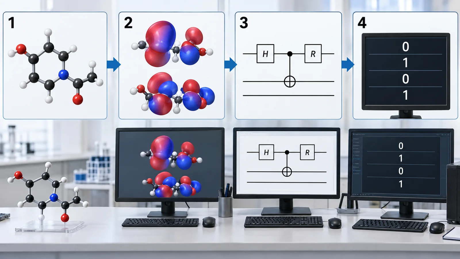
View original SVG, values and sources
Original SVG reference: Concept diagram (vector drawing). The flow of putting a molecular calculation on a quantum computer. Blue is the classical computer's work, orange the quantum computer's.
There are three broad ways to read out the energy (step 6). They differ in their dependence on error correction and in how reliable the result is.
| Method | How it works | Circuit length | Reliability of the result |
|---|---|---|---|
| Quantum phase estimation (QPE) | Reads the phase (rotation speed) of time evolution through interference to get the energy (Kitaev 1995; Abrams and Lloyd 1999) [Refs. 11, 12]Sourced | Long (error correction assumed) | Precision can be controlled theoretically; most scale estimates assume this method (chapter 7) |
| VQE | A classical computer tunes the knobs of a short circuit to lower the energy (see the NISQ explainer) [Refs. 14, 15]Sourced | Short (feasible on NISQ devices) | Heuristic; needs many measurements and offers weak accuracy guarantees (see the NISQ explainer) |
| Sample-based (SQD) | A quantum device samples electron configurations and a classical supercomputer diagonalizes a small subspace (Robledo-Moreno et al. 2025) [Ref. 17]Sourced | Relatively short | Gives an upper bound on the energy and a sparse wavefunction; some analyses find it less efficient than classical methods (chapter 6) |
The comparison of methods is this article's commentary (based on the statements in the references).
(1) Intuition for phase estimation: reading how fast the arrow turns
Phase estimation is easiest to grasp as reading the energy from how fast a clock hand turns. The arrow of a qubit turns over time at a speed proportional to the energy: the higher the energy, the faster the hand. Even two states with only slightly different energies can be told apart if run for long enough, because the angle between their hands grows.
A better precision requires a long time t and so a long circuit. Long circuits accumulate errors until the result is corrupted (see the NISQ explainer: even at a 0.1% error, 1,000 gates leave about a 37% success chance). Hence most estimates of the scale needed assume phase estimation on error-corrected logical qubits (chapter 7).
6. Molecules tried on real devices: scale and accuracy, without exaggeration
Here is how far the reasoning above has been tested on real devices, in chronological order. To state the conclusion first: the molecules tried on real devices are small, and most are of a size classical methods solve accurately. This is not a disappointment; it is fair to read it as a step-by-step check of device quality.
| Experiment | Device and scale | What was computed | Accuracy and reading notes |
|---|---|---|---|
| Lanyon et al. (2010) | Photonic | The energy of H₂ (minimal basis) by phase estimation | The smallest molecule; a proof of principle Sourced[Ref. 13] |
| Peruzzo et al. (2014) | Photonic (small) | Ground-state energy of HeH⁺ (VQE) | Reported within chemical accuracy; a tiny two-electron molecule Sourced[Ref. 14] |
| Kandala et al. (2017) | Superconducting, up to six qubits | Ground-state energies of H₂, LiH and BeH₂ (VQE) | Agreed with numerical simulation including device noise; small molecules classical methods solve exactly Sourced[Ref. 15] |
| Google (2020) | Superconducting, 12 qubits, 78 two-qubit gates | Binding energies of H₆ to H₁₂ chains and a model of diazene isomerization | The prepared state is the Hartree-Fock state, easy to find classically; the experiment tests the accuracy of orbital rotations Sourced[Ref. 16] |
| Robledo-Moreno et al. (2025) | IBM Heron (up to 77 qubits) + Fugaku | Ground states of N₂ (58 qubits), [2Fe-2S] (45) and [4Fe-4S] (77) | An upper bound on the energy and a sparse wavefunction; beyond the full-CI limit in size, but the quantum part supplies samples and the rest is classical Sourced[Ref. 17] |
| Yamamoto et al. (Quantinuum, 2025–2026) | Trapped-ion H2-2, encoded in the [[7,1,3]] color code | Ground-state energy of H₂ (QPE) | Presented as the first end-to-end demonstration of QPE with error correction. The difference from the exact value (within the basis) is 0.001(13) hartree, so the error bar (±0.013) is larger than chemical accuracy (0.0016) Sourced[Ref. 19] |
A summary of what each paper states (checked on 16 October 2026). Scales are as stated in the papers; approaches, error rates and the classical share differ, so do not rank them against each other.
Opinions on SQD (the sample-based method) are divided. Robledo-Moreno et al. state that even at current error rates, a quantum-centric supercomputing architecture can tackle chemistry problems beyond the size amenable to exact diagonalization Sourced[Ref. 17]. Reinholdt et al., on the other hand, analyse N₂ and [2Fe-2S] numerically and conclude that sample-based methods (QSCI and SQD) waste effort by repeatedly sampling configurations already seen, and fall behind more efficient classical methods Sourced[Ref. 18]. We do not judge which is right. Whether the method becomes practical needs results with the conditions matched against the best classical methods.
What the experiment yielded was an upper bound on the energy and a sparse approximation of the wavefunction Sourced[Ref. 17]. The quantum computer proposes "candidate" electron configurations by sampling, while the energy calculation itself is done by a classical supercomputer (Fugaku). The conditions of comparison with the best classical results for the same system must be checked paper by paper. The right reading: it is a first demonstration of a new quantum-classical arrangement, not "a quantum computer solved a molecule accurately".
7. Estimated scale needed: falling year by year, but still the future
How large a machine would a "practical molecule" need? Researchers have produced resource estimates (numbers of logical qubits and gates, and run time) assuming phase estimation on an error-corrected machine. The estimates have fallen year by year as algorithms improved. But an estimate is a calculation premised on a future machine, not the performance of any existing one.
| Study | Target | Estimate (as the paper states) | Conditions and cautions |
|---|---|---|---|
| Reiher et al. (2017) | FeMoco (the active centre of nitrogenase) | Concluded that even with error-correction overhead the calculation can run in reasonable time on small quantum computers [Ref. 20]Not yet confirmed | No figures in the abstract. The FeMoco active space is 54 electrons, 108 spin-orbitals (Lee et al.) |
| von Burg et al. (2021) | A ruthenium catalyst turning CO₂ into methanol | More than an order of magnitude better than previous algorithms [Ref. 22]Not yet confirmed | New algorithms for double-factorized representations |
| Lee et al. (2021) | FeMoco | About four million physical qubits and under four days [Ref. 21]Not yet confirmed | Assumes a 1 µs cycle time, physical gate errors no worse than 0.1% and the surface code; uses tensor hypercontraction (THC) |
| Goings et al. (2022) | Models of cytochrome P450 | Compared the convergence of classical DMRG and CCSD(T) with the resources of quantum phase estimation and concluded the models have the potential to be a quantum advantage problem [Ref. 23]Not yet confirmed | Based on estimates; notable for putting classical and quantum resources side by side |
| Caesura et al. (2025) | P450 and others | Estimated run time about two orders of magnitude shorter than prior-art algorithms [Ref. 24]Not yet confirmed | Estimates assume a photonic fault-tolerant machine (an active-volume layout) |
| Low et al. (2025) | Models of Fe–S complexes and a CO₂-fixation catalyst | Energy estimation 4 to 195 times faster than the state of the art [Ref. 25]Not yet confirmed | A new technique called spectrum amplification |
A summary of what each paper states. Resource estimates depend strongly on assumptions (cycle time, error rate, code). Checked on 16 October 2026.
That the estimates are falling is itself encouraging. But the timing of realisation is not settled. When and by which approach large error-corrected machines will arrive is outside this article and is covered in our explainers on logical qubits and fault tolerance and on national strategies Not yet confirmed.
8. Comparison with classical methods: opinions are divided
Researchers' views differ on whether quantum computers will beat classical ones in chemistry. The main positions are set out side by side.
| Position | Claim (as the paper states) | Reading |
|---|---|---|
| Cautious: Lee et al. (2023) | For ground-state energy estimation, evidence for exponential quantum advantage across chemical space has yet to be found. Quantum computers may still prove useful, but it may be prudent to assume exponential speedups are not generically available [Ref. 26]Sourced | Does not deny that polynomial or constant-factor gains could still matter |
| Targeted: Goings et al. (2022) | Compared P450 models through classical convergence analysis and quantum resource estimates and said they have the potential to be a quantum advantage problem [Ref. 23]SourcedNot yet confirmed | Based on specific systems and estimates; wording is "potential" |
| Practicality-focused: Hoefler et al. (2023) | Practical quantum advantage needs small-data problems and super-quadratic speedups. Most proposed applications do not meet this, but there is great potential in materials science and chemistry [Ref. 27]Sourced | A place among all applications; chemistry is a promising exception |
| Review: Bauer et al. (2020) | One cannot expect arbitrary simulations to be sped up, so areas where advantage may be achieved must be carefully identified [Ref. 6]Sourced | Premise: narrow down which problem |
A summary of what each paper states. It does not decide among them.
9. Materials simulation: lattice models and how they differ from molecules
The properties of materials (solids) are set by the behaviour of electrons just as in molecules, but because atoms sit in a periodic arrangement, they are often studied with a simple model of "electrons on a lattice". The best-known is the Hubbard model: electrons occupy sites and are governed by just two quantities, how easily they hop to a neighbouring site (t) and the repulsion when two share a site (U). The contest between the two is believed to give rise to behaviour such as magnetism and superconductivity.
- Lattice models map onto qubits more easily than molecular electronic structure and are listed among promising candidates for near-term experiments (the 2D Fermi-Hubbard model, spin models and others) Sourced[Refs. 5, 6]. In 2020 Google observed charge and spin spreading at different speeds in a 1D Hubbard model, using 16 qubits and over 600 two-qubit gates Sourced[Ref. 28].
- In 2026 Quantinuum reported in Nature that it observed the time evolution of an Ising model out to times that severely challenge classical simulation methods and computed a diffusion constant (two-qubit partial-entangler fidelity 99.94(1)%) Sourced[Ref. 29] (a company report).
- Both are experiments on how a model behaves, not measurements of an actual material's properties. How well the model represents a real material is a separate question (our commentary).
Google's Quantum Echoes (2025) presented a task for which measuring a physical quantity is estimated to take classical computers about 13,000 times longer. In the same line of work, an application combining the results with nuclear magnetic resonance (NMR) data to study molecular structure was shown in a separate, un-reviewed paper, but Google itself says "this initial demonstration is not yet beyond classical" Sourced[Ref. 30]. The tasks where advantage was shown and the tasks useful for molecules do not yet coincide (see the quantum advantage explainer).
10. A materials engineer's view
In the FeMoco example the target is a 54-electron, 54-orbital active space out of a huge enzyme containing iron, molybdenum, sulfur and more Sourced[Ref. 21]. The rest (the surrounding protein, solvent, structural fluctuations) is handled by classical methods. Translated to the materials floor, the picture is "the catalyst's active site on the quantum side, and the effects of support, solvent and temperature classically" (our commentary).
So when a materials engineer hears that "this can be computed on a quantum computer", three things should be checked. (1) Which active space: how many electrons and orbitals, and is it within reach of classical DMRG or CCSD(T)? (2) How the outside of the active space is treated: with what accuracy were structure, solvent and interfaces included? (3) Was it compared with experiment: even if the energy is right to chemical accuracy, it does not map directly onto what is measured.
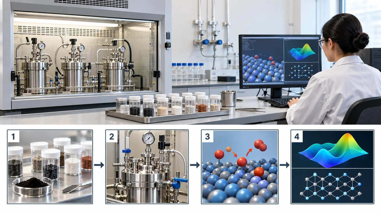
On the classical side too, fast methods such as machine-learning interatomic potentials are advancing rapidly (see our materials informatics explainers). In materials discovery, classical methods are strong for screening many candidates quickly, whereas quantum computers target calculating a few hard systems with high accuracy; the roles seem different (our commentary).
Another point: model errors often dominate before energy accuracy does. Differences in structure, solvent, temperature, interfaces and defects produce gaps with experiment independently of the accuracy of the electronic-structure calculation (our commentary). Even if a quantum computer reached chemical accuracy, agreement with experiment needs separate checking.
11. Limits, what we could not confirm, and a summary
(1) What we could not confirm
- We did not confirm the specific figures of the FeMoco estimate of Reiher et al. (2017); the abstract gives none.
- We do not give details such as qubit counts for Peruzzo et al. (2014) and Lanyon et al. (2010), as the abstracts do not state them.
- We did not confirm the size of the energy errors in the SQD experiments (the gap to the best classical results).
- We do not give cost formulas for DFT, DMRG and others beyond what we confirmed (about M⁷ for CCSD(T)).
- We found no third-party-verified case in which a real device computed a material's properties more accurately than the best classical methods.
- The text of ISO/IEC 4879:2024 is paywalled, so we could not confirm whether it covers quantum-chemistry terms. We did not find a standard defining the performance of quantum computers for chemistry and materials.
- The number of values for an exact calculation grows combinatorially with electrons (about 5×10¹¹ for 22 in 22, about 1.6×10²⁸ for 50 in 50). The limit of full CI is about 22 electrons in 22 orbitals Our calculationSourced
- A quantum computer uses one qubit per spin-orbital and reads the energy by phase estimation, VQE or sample-based methods. Phase estimation needs long circuits and assumes error correction Sourced
- The molecules tried on real devices are small, and most can be solved accurately classically. Even the largest SQD run (77 qubits) has the quantum part only sample configurations while the rest is classical; the error bar of the error-corrected H₂ run is larger than chemical accuracy Sourced
- Estimates of the scale needed have fallen year by year (about four million physical qubits and under four days for FeMoco, under stated assumptions), but the timing of realisation is not settled SourcedNot yet confirmed
- Whether quantum beats classical is disputed. The target is a few strongly correlated orbitals (the active space), and linking to measured material properties needs separate checking Sourced
12. How to read evaluations and standards
The first yardstick of quantum chemistry is energy accuracy (chemical accuracy, 1.6 mHa). Next come which classical method it is compared with (full CI, CCSD(T), DMRG and so on) and the resources needed (logical qubits, gates, run time). The chemical-accuracy target exists so that energy differences can be tied to predictions of reaction rates Sourced[Ref. 4]. Checked on 16 October 2026.
| Item | Representative benchmarks and methods (name, source) | Standards and guidance (ISO/IEC, NIST, DARPA, etc.) | Reading notes |
|---|---|---|---|
| Energy accuracy | Chemical accuracy (1.6×10⁻³ Ha); one definition requires it at every point of the potential energy surface (McArdle et al.) [Ref. 4]Sourced | Not found (we did not find an international standard defining chemical accuracy) | Requirements differ for absolute energies and energy differences; compare with error bars (see Yamamoto et al.) |
| Classical comparison data | NIST CCCBDB: experimental and computed thermochemical data for a selected set of 2,186 gas-phase atoms and small molecules (NIST Standard Reference Database 101) [Ref. 31]Sourced | A NIST standard reference database (not a standard) | Small-molecule data; not a baseline for large strongly correlated systems |
| Test problems for quantum algorithms | HamLib: an open library of Hamiltonians for benchmarking quantum algorithms and hardware (Sawaya et al. 2024) [Ref. 32]Sourced | Not found | Compare also with the best classical methods on the same problem |
| Resource estimation | Estimates in each paper (Lee et al., Goings et al., Caesura et al., Low et al.); estimation tools such as the Azure Quantum Resource Estimator (van Dam et al.) [Refs. 21, 23, 24, 25, 33]SourcedNot yet confirmed | Not found | Estimates depend strongly on assumptions about cycle time, error rate and code; plans, not achievements |
| Path to utility scale | DARPA QBI: utility scale = computational value exceeds cost; third-party verification and validation [Ref. 34]SourcedNot yet confirmed | A US government programme (not an international standard) | 2033 is DARPA's goal and estimate |
| Standardising terms and benchmarks | — | ISO/IEC 4879:2024 (quantum computing vocabulary, published May 2024) [Ref. 36]; ISO/IEC JTC 3/JSC 3A WG 2 on benchmarking [Ref. 35]SourcedNot yet confirmed | Text paywalled; we could not confirm any chemistry-specific terms or benchmarks |
The table's organisation is Our calculation (a summary). Numbers, titles and status were checked on the official ISO, NIST and DARPA pages (16 October 2026). Standards texts are paywalled, so we state only scope and no requirements.
Reading notes for materials engineers
- "How many qubits" does not tell you the molecule's size: the meaning of the count changes with the number of orbitals, the method and the classical share. The 77 qubits of the largest SQD run belong to an approach in which the quantum part is small [Ref. 17]
- Put error bars next to chemical accuracy: in the error-corrected H₂ example the error bar (±0.013 Ha) is larger than chemical accuracy (0.0016 Ha), so one cannot say the accuracy reached chemical accuracy [Refs. 19, 4]
- Separate plans from achievements: resource estimates, DARPA's 2033 and company roadmaps are goals and estimates. Many standards are still in development, and even once published they generally bind only when cited in law or contracts (our commentary) [Refs. 21, 34].
13. Glossary
- Electron correlation
- The way electrons avoid each other; the part a mean field cannot express.
- Dynamic / static correlation
- A small correction from electron repulsion / correlation arising when several arrangements are equally important.
- Orbital (spin-orbital)
- A "room" for an electron; a spin-orbital also distinguishes the spin direction (up/down).
- Basis set
- The set of functions used to describe orbitals; larger is more precise but costlier.
- Ground state
- The state of lowest energy.
- Chemical accuracy
- Energy error within 1.6 mHa (about 1 kcal/mol); the accuracy needed for predicting reaction rates.
- Hartree (Ha)
- A unit of energy: 1 Ha ≈ 27.2 eV ≈ 627.5 kcal/mol.
- Full CI (FCI)
- Solving exactly within the basis using every electron arrangement; the number of states grows combinatorially.
- Hartree-Fock (HF)
- An approximation in which each electron feels a mean field; ignores correlation.
- DFT (density functional theory)
- A widely used method that finds energies from the electron density.
- CCSD(T)
- A coupled-cluster method aiming at higher accuracy; time about M⁷.
- DMRG
- Density matrix renormalization group: a classical method that represents the state as a chain of small pieces.
- Active space
- The subset of electrons and orbitals with strong correlation that is treated with high accuracy.
- Strongly correlated system
- A system with strong correlation and highly entangled wavefunctions; common in catalysts and high-Tc superconductors.
- Jordan-Wigner mapping
- Mapping one spin-orbital to one qubit (0 = empty, 1 = occupied).
- Quantum phase estimation (QPE)
- Reading the energy from the phase (rotation speed) of time evolution; needs long circuits.
- VQE
- A method in which a classical computer tunes the knobs of a short circuit to lower the energy (for NISQ devices).
- SQD (sample-based quantum diagonalization)
- Diagonalizing a small subspace classically from configurations sampled on a quantum device.
- FeMoco
- The active centre of the nitrogen-fixing enzyme nitrogenase (iron, molybdenum, sulfur); a standard target.
- Hubbard model
- A model of electrons on a lattice governed only by hopping (t) and on-site repulsion (U).
- Resource estimation
- Estimating from a design the logical qubits, gates and time a calculation needs.
- Logical qubit
- One qubit protected from errors by many physical qubits.
- NISQ
- A mid-sized quantum computer that has errors and does not correct them.
14. References
- Feynman R. P. "Simulating physics with computers", Int. J. Theor. Phys. 21, 467–488 (1982), DOI 10.1007/BF02650179 — doi.org/10.1007/BF02650179
- Lloyd S. "Universal quantum simulators", Science 273, 1073–1078 (1996), DOI 10.1126/science.273.5278.1073 — doi.org/10.1126/science.273.5278.1073
- Aspuru-Guzik A. et al. "Simulated quantum computation of molecular energies", Science 309, 1704–1707 (2005), DOI 10.1126/science.1113479 — doi.org/10.1126/science.1113479
- McArdle S. et al. "Quantum computational chemistry", Rev. Mod. Phys. 92, 015003 (2020), DOI 10.1103/RevModPhys.92.015003 — doi.org/10.1103/RevModPhys.92.015003
- Cao Y. et al. "Quantum chemistry in the age of quantum computing", Chem. Rev. 119, 10856–10915 (2019), DOI 10.1021/acs.chemrev.8b00803 — doi.org/10.1021/acs.chemrev.8b00803
- Bauer B., Bravyi S., Motta M., Chan G. K.-L. "Quantum algorithms for quantum chemistry and quantum materials science", Chem. Rev. 120, 12685–12717 (2020), DOI 10.1021/acs.chemrev.9b00829 — doi.org/10.1021/acs.chemrev.9b00829
- Hohenberg P., Kohn W. "Inhomogeneous electron gas", Phys. Rev. 136, B864–B871 (1964), DOI 10.1103/PhysRev.136.B864 — doi.org/10.1103/PhysRev.136.B864
- Kohn W., Sham L. J. "Self-consistent equations including exchange and correlation effects", Phys. Rev. 140, A1133–A1138 (1965), DOI 10.1103/PhysRev.140.A1133 — doi.org/10.1103/PhysRev.140.A1133
- Cohen A. J., Mori-Sánchez P., Yang W. "Challenges for density functional theory", Chem. Rev. 112, 289–320 (2012), DOI 10.1021/cr200107z — doi.org/10.1021/cr200107z
- White S. R. "Density matrix formulation for quantum renormalization groups", Phys. Rev. Lett. 69, 2863–2866 (1992), DOI 10.1103/PhysRevLett.69.2863 — doi.org/10.1103/PhysRevLett.69.2863
- Kitaev A. Yu. "Quantum measurements and the Abelian stabilizer problem", arXiv:quant-ph/9511026 (1995) — arxiv.org/abs/quant-ph/9511026
- Abrams D. S., Lloyd S. "Quantum algorithm providing exponential speed increase for finding eigenvalues and eigenvectors", Phys. Rev. Lett. 83, 5162–5165 (1999), DOI 10.1103/PhysRevLett.83.5162 — doi.org/10.1103/PhysRevLett.83.5162
- Lanyon B. P. et al. "Towards quantum chemistry on a quantum computer", Nat. Chem. 2, 106–111 (2010), DOI 10.1038/nchem.483 — doi.org/10.1038/nchem.483
- Peruzzo A. et al. "A variational eigenvalue solver on a quantum processor", Nat. Commun. 5, 4213 (2014), DOI 10.1038/ncomms5213 (open access) — doi.org/10.1038/ncomms5213
- Kandala A. et al. "Hardware-efficient variational quantum eigensolver for small molecules and quantum magnets", Nature 549, 242–246 (2017), DOI 10.1038/nature23879 — doi.org/10.1038/nature23879
- Google AI Quantum and collaborators "Hartree-Fock on a superconducting qubit quantum computer", Science 369, 1084–1089 (2020), DOI 10.1126/science.abb9811 — doi.org/10.1126/science.abb9811
- Robledo-Moreno J. et al. "Chemistry beyond the scale of exact diagonalization on a quantum-centric supercomputer", Sci. Adv. 11, eadu9991 (2025), arXiv:2405.05068 — arxiv.org/abs/2405.05068
- Reinholdt P. et al. "Critical limitations in quantum-selected configuration interaction methods", J. Chem. Theory Comput. 21, 6811–6822 (2025), arXiv:2501.07231 — arxiv.org/abs/2501.07231
- Yamamoto K. et al. (Quantinuum) "Quantum error-corrected computation of molecular energies", PRX Quantum (2026), arXiv:2505.09133 — arxiv.org/abs/2505.09133
- Reiher M. et al. "Elucidating reaction mechanisms on quantum computers", Proc. Natl. Acad. Sci. USA 114, 7555–7560 (2017), DOI 10.1073/pnas.1619152114 — doi.org/10.1073/pnas.1619152114
- Lee J. et al. "Even more efficient quantum computations of chemistry through tensor hypercontraction", PRX Quantum 2, 030305 (2021), DOI 10.1103/PRXQuantum.2.030305 — arxiv.org/abs/2011.03494
- von Burg V. et al. "Quantum computing enhanced computational catalysis", Phys. Rev. Research 3, 033055 (2021), DOI 10.1103/PhysRevResearch.3.033055 — doi.org/10.1103/PhysRevResearch.3.033055
- Goings J. J. et al. "Reliably assessing the electronic structure of cytochrome P450 on today's classical computers and tomorrow's quantum computers", Proc. Natl. Acad. Sci. USA 119, e2203533119 (2022), DOI 10.1073/pnas.2203533119 — doi.org/10.1073/pnas.2203533119
- Caesura A. et al. "Faster quantum chemistry simulations on a quantum computer with improved tensor factorization and active volume compilation", PRX Quantum 6, 030337 (2025), arXiv:2501.06165 — arxiv.org/abs/2501.06165
- Low G. H. et al. "Fast quantum simulation of electronic structure by spectrum amplification", Phys. Rev. X 15, 041016 (2025), arXiv:2502.15882 — arxiv.org/abs/2502.15882
- Lee S. et al. "Evaluating the evidence for exponential quantum advantage in ground-state quantum chemistry", Nat. Commun. 14, 1952 (2023), DOI 10.1038/s41467-023-37587-6 (open access) — doi.org/10.1038/s41467-023-37587-6
- Hoefler T., Häner T., Troyer M. "Disentangling hype from practicality: on realistically achieving quantum advantage", Commun. ACM 66(5), 82–87 (2023), DOI 10.1145/3571725 — doi.org/10.1145/3571725
- Google AI Quantum and collaborators "Observation of separated dynamics of charge and spin in the Fermi-Hubbard model", arXiv:2010.07965 (2020) — arxiv.org/abs/2010.07965
- Haghshenas R. et al. (Quantinuum) "Digital quantum magnetism on a trapped-ion quantum computer", Nature 653, 56–62 (2026), DOI 10.1038/s41586-026-10445-3 — nature.com/articles/s41586-026-10445-3
- Google Quantum AI "A verifiable quantum advantage" (Google Research blog, 22 October 2025) — research.google/blog/a-verifiable-quantum-advantage/
- NIST "Computational Chemistry Comparison and Benchmark DataBase (CCCBDB)", NIST Standard Reference Database 101 — cccbdb.nist.gov
- Sawaya N. P. D. et al. "HamLib: a library of Hamiltonians for benchmarking quantum algorithms and hardware", Quantum 8, 1559 (2024), DOI 10.22331/q-2024-12-11-1559 — doi.org/10.22331/q-2024-12-11-1559
- van Dam W., Mykhailova M., Soeken M. "Using Azure Quantum Resource Estimator for assessing performance of fault tolerant quantum computation", arXiv:2311.05801 (2023) — arxiv.org/abs/2311.05801
- DARPA "Quantum Benchmarking Initiative (QBI)" (program page; list current as of 8 October 2026) — darpa.mil/research/programs/quantum-benchmarking-initiative
- IEC/ISO JTC 3/JSC 3A "Quantum computing" (committee page: scope and working groups, including WG 2 benchmarking) — iso.org/committee/12010875.html
- ISO/IEC "ISO/IEC 4879:2024 Information technology — Quantum computing — Vocabulary" (ISO catalogue page) — iso.org/standard/80432.html
15. Claim-to-source audit
| Claim in the text | Basis | Category |
|---|---|---|
| Feynman's 1982 argument that quantum systems call for a computer with quantum properties; Lloyd's universal quantum simulators (1996); Aspuru-Guzik et al.'s proposal for molecular energies (2005) | Reference 1 https://doi.org/10.1007/BF02650179 Reference 2 https://doi.org/10.1126/science.273.5278.1073 Reference 3 https://doi.org/10.1126/science.1113479 | Sourced |
| Chemical accuracy of 1.6×10⁻³ hartree and prediction of room-temperature rates to within an order of magnitude; HF neglecting dynamic and static correlation; the definition of static correlation; strongly correlated systems having highly entangled wavefunctions, with catalysts and high-temperature superconductors as examples; CCSD(T) time about M⁷; the basic Jordan-Wigner mapping (one spin-orbital = one qubit) | Reference 4 https://doi.org/10.1103/RevModPhys.92.015003 | Sourced |
| The review of quantum chemistry (Cao et al.); the review of chemistry and materials: one cannot expect arbitrary simulations to be sped up and must identify where advantage may be achieved, and lattice models being near-term candidates (Bauer et al.) | Reference 5 https://doi.org/10.1021/acs.chemrev.8b00803 Reference 6 https://doi.org/10.1021/acs.chemrev.9b00829 | Sourced |
| The foundations of DFT (Hohenberg and Kohn; Kohn and Sham), the review of DFT challenges (Cohen et al.), and the proposal of DMRG (White) | Reference 7 https://doi.org/10.1103/PhysRev.136.B864 Reference 8 https://doi.org/10.1103/PhysRev.140.A1133 Reference 9 https://doi.org/10.1021/cr200107z Reference 10 https://doi.org/10.1103/PhysRevLett.69.2863 | Sourced |
| The foundations of phase estimation (Kitaev 1995; Abrams and Lloyd 1999) | Reference 11 https://arxiv.org/abs/quant-ph/9511026 Reference 12 https://doi.org/10.1103/PhysRevLett.83.5162 | Sourced |
| Lanyon et al.: the energy of H₂ on a photonic device; Peruzzo et al.: HeH⁺ within chemical accuracy; Kandala et al.: H₂, LiH and BeH₂ with up to six qubits (agreeing with noisy numerical simulation) | Reference 13 https://doi.org/10.1038/nchem.483 Reference 14 https://doi.org/10.1038/ncomms5213 Reference 15 https://doi.org/10.1038/nature23879 | Sourced |
| Google's 12-qubit experiment: H₆ to H₁₂ chains, diazene isomerization, preparation of the Hartree-Fock state, 78 two-qubit gates | Reference 16 https://doi.org/10.1126/science.abb9811 | Sourced |
| SQD: N₂ (58 qubits), [2Fe-2S] (45) and [4Fe-4S] (77), up to 10,570 gates, Fugaku, an upper bound on the energy and a sparse wavefunction, and the statement that the full-CI limit is about 22 electrons in 22 orbitals and 26 in 23 | Reference 17 https://arxiv.org/abs/2405.05068 | Sourced |
| Reinholdt et al.: QSCI and SQD resample configurations already seen and fall behind more efficient classical methods (N₂, [2Fe-2S]) | Reference 18 https://arxiv.org/abs/2501.07231 | Sourced |
| Yamamoto et al. (Quantinuum): the H₂ energy by QPE encoded in the [[7,1,3]] color code, 0.001(13) hartree from the exact value | Reference 19 https://arxiv.org/abs/2505.09133 | Sourced |
| Reiher et al.: the FeMoco estimate (reasonable time on small quantum computers even with error-correction overhead) | Reference 20 https://doi.org/10.1073/pnas.1619152114 | Sourced |
| Lee et al. (2021): about four million physical qubits and under four days for FeMoco (1 µs cycle, errors at most 0.1%); 54 electrons and 108 spin-orbitals | Reference 21 https://arxiv.org/abs/2011.03494 | Sourced |
| von Burg et al.: more than an order of magnitude improvement for a ruthenium catalyst | Reference 22 https://doi.org/10.1103/PhysRevResearch.3.033055 | Sourced |
| Goings et al.: compared classical DMRG and CCSD(T) with quantum resources for P450 models and said they have the potential to be a quantum advantage problem | Reference 23 https://doi.org/10.1073/pnas.2203533119 | Sourced |
| Caesura et al.: estimated run time about two orders of magnitude shorter than prior art; Low et al.: 4 to 195 times speed-up for Fe–S complexes and a CO₂-fixation catalyst | Reference 24 https://arxiv.org/abs/2501.06165 Reference 25 https://arxiv.org/abs/2502.15882 | Sourced |
| Lee et al. (2023): no evidence yet of exponential quantum advantage across chemical space; Hoefler et al.: the conditions for practical quantum advantage and the potential of materials science and chemistry | Reference 26 https://doi.org/10.1038/s41467-023-37587-6 Reference 27 https://doi.org/10.1145/3571725 | Sourced |
| Google's 1D Hubbard-model experiment (16 qubits, over 600 two-qubit gates); Quantinuum's Ising-model time evolution (Nature 2026, partial-entangler fidelity 99.94(1)%) | Reference 28 https://arxiv.org/abs/2010.07965 Reference 29 https://www.nature.com/articles/s41586-026-10445-3 | Sourced |
| Google's statement that the molecular application of Quantum Echoes is "not yet beyond classical", and the 13,000-times estimate (company claims) | Reference 30 https://research.google/blog/a-verifiable-quantum-advantage/ | Sourced |
| NIST CCCBDB (2,186 gas-phase atoms and small molecules); HamLib (an open library of benchmark Hamiltonians); the Azure Quantum Resource Estimator | Reference 31 https://cccbdb.nist.gov Reference 32 https://doi.org/10.22331/q-2024-12-11-1559 Reference 33 https://arxiv.org/abs/2311.05801 | Sourced |
| DARPA QBI's definition of utility scale and its 2033 estimate (participants as of 8 October 2026) | Reference 34 https://www.darpa.mil/research/programs/quantum-benchmarking-initiative | Sourced |
| WG 2 (benchmarking) of ISO/IEC JTC 3/JSC 3A; ISO/IEC 4879:2024 number, title and May 2024 publication | Reference 35 https://www.iso.org/committee/12010875.html Reference 36 https://www.iso.org/standard/80432.html | Sourced |
| The full-CI dimensions (C(n, n/2)²: 10 → 6.4×10⁴, 18 → 2.4×10⁹, 22 → 5.0×10¹¹, 30 → 2.4×10¹⁶, 50 → 1.6×10²⁸, 54 → 3.8×10³⁰), memory (double precision), 2n qubits, 1.6 mHa ≈ 1.0 kcal/mol ≈ 4.2 kJ/mol ≈ 0.044 eV, kT ≈ 0.596 kcal/mol at 300 K, a 5.4-fold rate change per 1 kcal/mol and about 2×10⁷ at 16 mHa | Our calculation (Python, standard conversion constants) | Our calculation |
| The specific figures of Reiher et al.'s estimate, the qubit counts of Peruzzo et al. and Lanyon et al., the size of the SQD energy errors, cost formulas for DFT and DMRG, third-party-verified quantum advantage on material properties, quantum-chemistry terms in ISO/IEC 4879, and performance standards for chemistry and materials | Not confirmed in the primary sources reachable for this article, so not stated | Commentary |
| The readings: the classical/quantum division of labour (the active space), "the target is a few strongly correlated orbitals", model errors on the materials floor, the different roles of classical AI methods, and "lattice models are distinct from real materials" | This article's commentary based on published material; not views stated by the institutions | Commentary |
| Fig. 3 and Fig. 7 are illustrations (calculations) rather than real data; Fig. 2, Fig. 4, Fig. 5, Fig. 6, Fig. 8 and Fig. 9 are concept diagrams; Fig. 1 and Fig. 10 are ImageGen-generated conceptual illustrations | A note in this article | Commentary |
Last updated: 16 October 2026. Sources are limited to primary material (peer-reviewed papers, arXiv papers, Google's official blog, official NIST, DARPA and ISO pages). Numerical examples are our own calculations, not device results. We could not confirm the specific figures of the estimate by Reiher et al., the size of the SQD energy errors, cost formulas for DFT and DMRG, third-party-verified quantum advantage on material properties, or quantum-chemistry terms in ISO/IEC 4879, so we do not state them. All figures are illustrative concept diagrams or drawings that include our calculations; Fig. 1 and Fig. 10 are ImageGen-generated conceptual illustrations.