TECHNOLOGY EXPLAINER
Fundamentals of Robot Control
– Robots move by “measure, correct, look ahead”
A robot is not a machine that moves just because you tell it “go there”. It reaches the intended motion only by measuring what actually happened and correcting the error, hundreds of times a second. For materials engineers new to control, this article explains six ideas with figures and small numerical examples: PID control, inverse kinematics, trajectory planning, model predictive control (MPC), impedance control and balance control. Equations are kept to a minimum; the emphasis is on “what problem each idea solves, and how”. The later part deals with where control meets materials and parts – structural resonance, reducers and sensors – which set the limits of control.
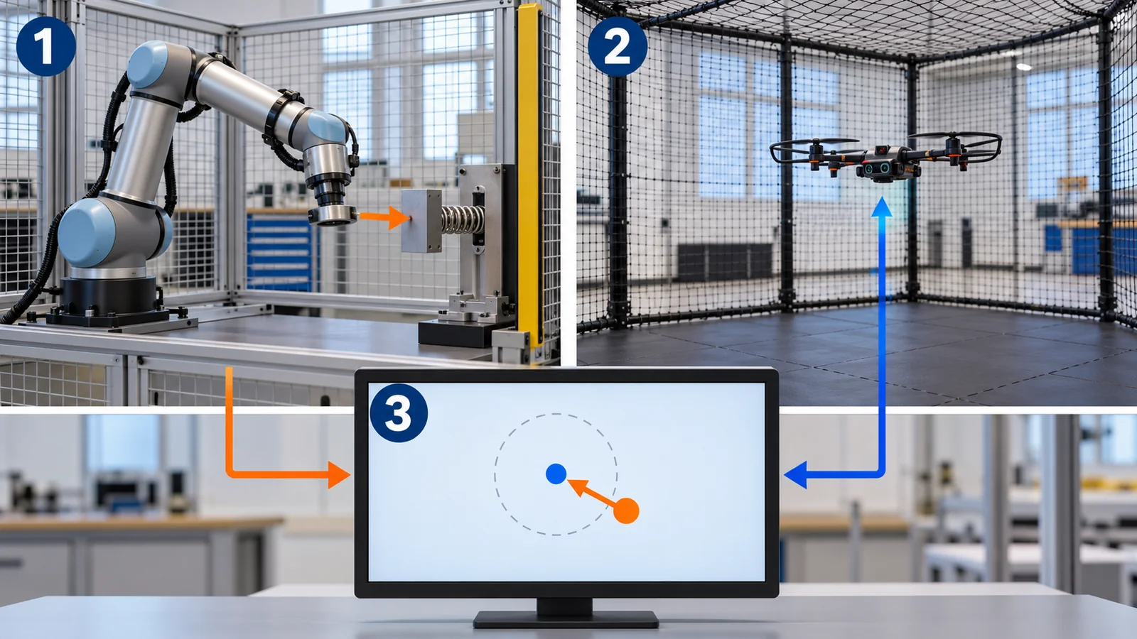
- What is robot control? (the short version)
- Measure and correct: feedback and PID
- From tip position to joint angles: inverse kinematics
- How to move: trajectory planning
- Looking ahead: model predictive control (MPC)
- Touching with force: impedance control
- Standing without falling: balance control
- Materials and parts set the limits of control
- Limits, what we could not confirm, and a summary
- How to read the yardsticks and standards
- Glossary
- References (primary sources)
- Claim-to-source audit
Sourced = stated in a published source (linked)
Our calculation = our own calculation or simulation (assumptions are stated)
Not yet confirmed = drafts or work in progress that is not settled
Inference is shown in bold. Readings that have no source are marked “commentary”.
The curves and numbers in Chapters 2 to 7 come from simple models we made, simulated or calculated ourselves. They do not describe the performance or gain values of any real robot, and they are not a recipe for “set it like this”. Manufacturer numbers are written as “company’s stated values”. Results from papers are for the conditions of those papers. For standards we only checked number, title and status, not the text. We give no individual safety advice.
1. What is robot control? (the short version)
- Control is repeating “measure, then correct”: measure the gap between the target and the actual value, and apply force in the direction that shrinks it. This is called feedback. A textbook says that PID control is by far the most common design technique, and that more than 95% of industrial control problems are solved by PID [Ref. 2] Sourced.
- Control is built in layers: for a robot arm the layers are “plan, inverse kinematics, servo”; for a drone, “position, velocity, attitude, angular rate”. The outer layers set goals and the inner layers produce force, nested like boxes (Fig. 2).
- MPC, impedance and balance sit on this base: “look ahead”, “touch with force” and “stand without falling” are different tools, but all of them rest on “measure and correct”.
In this series a robot is a combination of three things: “sense” (sensors), “think” (control and intelligence) and “move” (actuators). The star of this article is the part of “think” that makes motion accurate: control. Degrees of freedom (DOF) are the number of directions in which a joint can move. A gain is a coefficient for how strongly to correct a given error.
Where this fits in the series: the parts that move joints are in our explainers on joint actuators and on reducers and gears, the stiffness of the body in the one on structural materials for robots and drones, force measurement in the one on tactile sensors and electronic skin, learned motion in the one on imitation and reinforcement learning, and safety standards in the one on reading robot safety standards. This article covers the classical control underneath them.
2. Measure and correct: feedback and PID
A familiar comparison is adjusting a shower’s temperature. You feel the water, add cold if it is too hot and hot if it is too cool. Measure, then correct the error – that is feedback. A robot joint likewise measures its angle with an encoder (an angle sensor) and adjusts the motor force to shrink the gap to the target.
The most basic form of this adjustment is PID control. It decides the force u sent to the motor from the error e in three ways.
u = Kp x e + Ki x (accumulated e) + Kd x (rate of change of e)
- P (proportional): the larger the present error, the harder it corrects. In the shower: “the hotter it is, the more cold water I add”.
- I (integral): the longer the error lingers, the harder it corrects (it looks at the accumulated error). “The temperature still isn’t right, so I turn the tap a bit more.”
- D (derivative): if the error is shrinking quickly, ease off early (it looks at how the error is changing). “It’s getting close, so I start turning the tap back” (the comparison’s limit: the real D term is sensitive to noise).
A numerical example: how much the gains change the motion
We ran a simple simulation of a joint with inertia J = 0.05 kg·m² moving to a target of 1 rad (about 57 degrees) Our calculation. The D term acts on velocity (PD control), and we compare three gain sets (Fig. 3, top). A (Kp 5) is slow, taking about 0.69 s to settle within 2%, with no overshoot. B (Kp 50) settles in about 0.19 s with an overshoot of about 6%. C (Kp 500) is faster still, but overshoots by about 51% and oscillates a few times, settling in about 0.17 s Our calculation. Raising the gain makes it faster, but raising it too far makes it oscillate.
The bottom of Fig. 3 shows a constant force such as gravity acting all the time. Facing a gravity torque of 0.5 N·m with PD control at Kp 50 leaves an offset of 0.01 rad (about 0.57 degrees) Our calculation (0.5 / 50 = 0.01), because the force proportional to that offset is exactly what balances gravity. Adding I (integral) makes the accumulated error keep raising the force, so the offset vanishes Our calculation.
The I term grows large if the error persists. If the motor force has a limit (saturation), the accumulated integral keeps pushing after the target is reached and causes overshoot. This is called integrator windup, and the textbook explains that a countermeasure called “anti-windup” is needed [Ref. 2] Sourced. For robots with limited motor force it is always a concern.
Drones are nested PIDs too
The PX4 documentation (drone flight-control software) describes multicopter control as a cascaded (nested) structure [Ref. 3] Sourced. A P controller on position commands velocity, and a PID on velocity commands acceleration (tilt). A P controller on attitude commands angular rate, and the innermost angular-rate loop is made of three PID controllers, for roll, pitch and yaw [Ref. 3, 4] Sourced. If this inner loop is badly tuned, the documentation says, the aircraft will “twitch” or oscillate even in position-hold modes [Ref. 4] Sourced.
As curve C in Fig. 3 shows, too much gain overshoots and oscillates. On a real machine there are also sensor noise, delays in communication and computation, and structural resonance, and raising the gain makes it easier to go unstable (commentary; structural resonance is in Chapter 8). The correct reading: you choose the gain as a trade-off among speed, overshoot and robustness to noise and delay.
3. From tip position to joint angles: inverse kinematics
When you tell a robot “put the hand here”, the controller must compute what angle each joint should take. Finding the tip position from the joint angles is “forward kinematics”, an easy calculation. The reverse – finding the joint angles from the tip position – is inverse kinematics. Modern Robotics explains that for a given set of joint positions the tip pose is unique, but for a given tip pose there can be several joint solutions, or none [Ref. 1] Sourced.
We check with the simplest case, a planar arm with two links. Take link lengths of 0.40 m and 0.30 m and a tip target of (0.50, 0.20) m. The squared distance to the tip is 0.29 m². From the law of cosines, cos θ2 = (0.29 – 0.16 – 0.09) / (2 x 0.40 x 0.30) = about 0.167, so θ2 = ±80.4 degrees: two solutions Our calculation (Fig. 4). One has the elbow down (θ1 = -11.5 degrees, θ2 = +80.4 degrees), the other the elbow up (θ1 = +55.1 degrees, θ2 = -80.4 degrees) Our calculation. Modern Robotics too calls the two solutions “elbow-up” and “elbow-down” [Ref. 1] Sourced.
When the arm is nearly straight (θ2 close to 0), pulling the tip back along the arm is easy, but moving it at right angles to the arm can no longer be done with small joint motions. This state is called a singularity [Ref. 1]. In numbers, to move the tip at 1 m/s the joint speed needed in the worst direction is about 4.9 rad/s at θ2 = 80 degrees but about 36 rad/s at θ2 = 10 degrees, about 7.4 times as much Our calculation (Fig. 4, right). Beyond the maximum speed of the joint motors and reducers, the tip cannot move as commanded. It is like how, with your arm stretched out fully, you can hardly move it quickly sideways (the comparison’s limit: a human arm has many joints and avoids singularities more easily).
Modern Robotics explains that common six-degree-of-freedom arms have closed-form (analytic) solutions for inverse kinematics, and that for general arms the problem is solved iteratively by numerical computation using the Jacobian (the relation between joint motion and tip motion) [Ref. 1] Sourced.
4. How to move: trajectory planning
Knowing the tip target is not enough; you need which route, at what speed. A route alone is a “path”; a path with times assigned is a “trajectory” (commentary). Finding a path that avoids obstacles is “motion planning”, and there is research on methods that scatter random points to search for a route (sampling-based). Karaman and Frazzoli analyzed the quality of solutions from methods such as RRT and PRM and proposed RRT* and PRM*, which are provably asymptotically optimal [Ref. 10] Sourced.
A numerical example: a trapezoidal velocity profile
The most basic trajectory for one joint is the trapezoidal velocity profile. Modern Robotics explains that this “accelerate, cruise, decelerate” motion, whose velocity graph is a trapezoid, gives the fastest straight-line motion when the joint maximum velocity and acceleration are fixed [Ref. 1] Sourced.
Let us calculate. Move 2 rad with a maximum velocity of 2 rad/s and a maximum acceleration of 4 rad/s². Accelerating takes 2 / 4 = 0.5 s, covering 0.5 rad. Decelerating is the same 0.5 rad, and the cruise part is 2 – 0.5 – 0.5 = 1 rad, which at 2 rad/s takes 0.5 s. The total is 1.5 s Our calculation (Fig. 5). When the move is smaller and the maximum velocity is never reached, the profile becomes a triangle: accelerate, then immediately decelerate [Ref. 1] Sourced.
The trapezoidal trajectory is fast, but acceleration switches instantly (the corners at the bottom of Fig. 5). Modern Robotics notes that the trapezoidal time scaling is not as smooth as a cubic one [Ref. 1] Sourced. At the instant of switching, structures and cables get shaken and vibration can appear (commentary). For flexible robots or robots that swing a load, smoothness is sometimes chosen over speed.
5. Looking ahead: model predictive control (MPC)
PID reacts to “the present error”. MPC (Model Predictive Control) predicts a short stretch of the future with a model and decides the force to apply now. At each step it (1) predicts the coming motion, (2) finds the best sequence of forces within constraints such as force limits, and (3) executes only the first of them, then returns to (1) (Fig. 6, left). A familiar comparison is looking ahead in chess: you read a few moves ahead, choose the move now, watch the reply, and read again (the comparison’s limit: MPC’s “reading” is a calculation with a physical model and cannot read an opponent’s intent).
A numerical example: when force has a limit
Move a point mass from 0 to a position 1 m away. The acceleration limit is 1 m/s² (like a motor with limited force). PD control (Kp 4, Kd 2) approaches while stuck at the limit and overshoots by about 15% Our calculation. A PD with lower gains to remove the overshoot (Kp 1, Kd 2) takes about 5.85 s to settle within 2% Our calculation. The MPC (2 s look-ahead) starts decelerating early, so overshoot is about 1.9% and it settles in about 1.75 s Our calculation (Fig. 6, right). That is the effect of looking ahead when there are limits.
Two real-machine examples. Sun et al. compared nonlinear MPC (NMPC) with a differential-flatness-based controller for quadrotor tracking in agile flight up to 20 m/s (72 km/h), in simulation and on real aircraft [Ref. 8] Sourced. They conclude that NMPC is better at tracking trajectories that are hard to realize, at the cost of longer computation time and a risk of numerical convergence problems [Ref. 8] Sourced. Adding an inner-loop controller and an aerodynamic drag model cut the tracking error of both by more than 78% [Ref. 8] Sourced. Kuindersma et al. report building walking for the Atlas humanoid, from footstep placement to whole-body planning and control, using optimization tools such as convex optimization, mixed-integer programming and nonlinear optimization [Ref. 9] Sourced.
MPC is strong on problems with constraints or problems that need look-ahead, but it is computationally heavy, its performance drops if the model is inaccurate, and it cannot be used if computation does not keep up. In the comparison by Sun et al., NMPC pays with computation time and convergence risk [Ref. 8]. In real robots, a configuration with a low-level controller such as PID inside the MPC is common (commentary; the drone hierarchy in Chapter 2 is one example). The correct reading: it is not which is better; you use each for the problem at hand.
6. Touching with force: impedance control
So far we talked about moving “position” accurately. A robot that touches people and objects must also handle force. When pushing on a wall, fitting a part or bumping into a person, holding position too rigidly makes a large force the instant it meets something hard.
Impedance control makes the robot’s tip behave as if tied by a virtual spring (K) and damper (B) (Fig. 7, left). Modern Robotics explains that the aim is to make the robot act as having a chosen mass, spring and damper [Ref. 1] Sourced. Because it produces a force F = K x error, a softer spring (smaller K) gives a smaller force for the same error.
In numbers: for an error of 2 cm pushing into a wall, K = 500 N/m gives 10 N and K = 5000 N/m gives 100 N Our calculation (F = K x 0.02 m, Fig. 7, right). The K values are illustrative. It shows that with the same robot, one setting changes the force on contact by a factor of ten.
Modern Robotics distinguishes impedance control (measure motion, produce force) from admittance control (measure force, decide motion) [Ref. 1] Sourced. A classic paper on impedance control is Hogan (1985), “Impedance Control: An Approach to Manipulation” [Ref. 7] (we checked only its bibliographic record and do not cite its content).
Lowering K in impedance control does not by itself guarantee safety. If the control software fails, a sensor breaks or communication is delayed, the intended softness cannot be kept. Safety-related control is designed in a different way. ISO 13849-1:2023 sets a methodology for designing the safety-related parts of control systems and says that it does not itself specify the safety functions or required performance levels for particular applications [Ref. 16] Sourced. The technical specification on collaborative robots, ISO/TS 15066:2016, covers industrial robot systems [Ref. 15] Sourced (see our explainer on reading robot safety standards).
7. Standing without falling: balance control
A robot that walks on legs is on the verge of falling even when it just stands. A comparison is balancing a stick upright on your palm: unless you keep moving the base (your hand) in the direction the stick tips, it falls. A simplified model of this “inverted pendulum” is the linear inverted pendulum model, widely used in research on humanoid walking (Kajita et al. [Ref. 5]; we checked only the name and the fact of the proposal).
In this model, when no force is applied at the ankle, the offset x of the center of mass grows as x(t) = x0 x cosh(ωt), with ω = √(g / z) (g is gravitational acceleration, z the height of the center of mass) Our calculation. The meaning: the higher the center of mass, the slower the fall. With a center-of-mass height of 0.9 m, ω = 3.3 rad/s, and the starting offset doubles in about 0.40 s Our calculation. It is about 0.30 s at 0.5 m and about 0.51 s at 1.5 m Our calculation (Fig. 8). In other words, a robot about as tall as a person, left alone, doubles its offset in roughly 0.4 s, so it must keep correcting every instant by choosing where to place its feet and by using ankle and trunk forces.
A classic idea in balance control is the ZMP (zero-moment point): the point where the force under the foot produces no moment about the floor. While this point stays inside the sole, the foot does not rotate off the floor and fall. Vukobratović and Borovac published a paper summarizing 35 years of the ZMP (2004) [Ref. 6] Sourced (we checked only its title and bibliographic record).
ISO/CD 25785-1 is under development as a standard for the safety of robots whose stability is actively controlled (legged, self-balancing wheeled and so on). The ISO page says “a draft is being reviewed by the committee” and defines such a robot as one that “requires an active control in order to remain balanced and could become unstable in the absence of power” [Ref. 17] Sourced Not yet confirmed. As of the check date it is not a settled standard.
8. Materials and parts set the limits of control
The control above silently assumed “an ideal motor and an arm that does not deform”. In real robots, the properties of materials and parts set the limits of what control can do.
1. Structural resonance: stiffness decides the usable gain
Frames and arms have some elasticity like a spring, so they shake easily at particular frequencies (resonance). If the control bandwidth (the frequency range the control can follow) approaches a resonance, control excites the resonance and it vibrates. Milenin (2026) measured the resonance peaks of a 7-inch multicopter with a cast magnesium AZ31 frame at 147 Hz with no payload and 204 Hz with 2 kg, and for a 6061-T6 aluminum frame at 179.5 Hz and 239.4 Hz [Ref. 11] Sourced. The frame material and the payload move the resonance frequency (Fig. 9). The PX4 documentation explains that the gyro signal is processed with a notch filter (which cuts only a particular frequency) and a low-pass filter (which gently rolls off high frequencies) before control uses it [Ref. 4] Sourced.
The resonance frequency is roughly proportional to the square root of stiffness divided by the square root of mass (commentary; the “specific stiffness”, elastic modulus E divided by density rho, matters). As seen in our explainer on structural materials for robots and drones, a carbon-fiber composite with high specific stiffness can move the resonance to a higher frequency at the same mass. The higher the resonance, the wider the range of frequencies control can use, so gains can be raised and the motion made faster and more accurate (commentary). Damping (vibration absorption) of the material also matters. Milenin (2026) reports that the magnesium frame had 49% less vibration power than the aluminum aircraft (2 kg payload, one particular design) [Ref. 11] Sourced. Lightening concerns not only mass but also the limits of control.
2. Friction, backlash and sensors: the properties of the parts control relies on
The backlash (play in gear meshing) and friction of reducers (gears) are why control does not work as intended where the error is small. The “remaining offset” in the bottom of Fig. 3 is also caused by a constant force such as friction. The resolution and noise of the encoder (angle sensor) set the quality of the D term (which looks at the rate of change) (commentary; reducers are in our explainer on reducers and gears).
As seen in our explainer on structural materials for robots and drones, motors of a CFRP-framed aircraft exceeded 90 °C under payload (Milenin, 2025 [Ref. 18] Sourced). A motor’s winding resistance and magnet strength change with temperature, so the same current gives a different torque (commentary). If the controller assumes design-time values, the hotter it gets, the less force it produces as intended. So measures such as measuring motor temperature and compensating, or holding temperature down with materials and heat-removal design, support control accuracy (Inference).
3. Soft robots: the assumptions of control break down
The electrohydraulic leg seen in our explainer on soft robots and artificial muscles has a dead zone (0 to 3 kV) in which it does not respond to voltage, and it combined PID at a low level with open-loop control that leaves work to the softness of the body. It is an example where the classical assumptions “linear, and does not deform” cannot be used as they are.
9. Limits, what we could not confirm, and a summary
What we could not confirm
- Servo loop rates (Hz) of industrial and humanoid robots: we did not find a manufacturer’s official document giving the control-loop rate. The PX4 documentation did not give rate numbers we could confirm either
- The content of Hogan (1985): we checked only the bibliographic record, not the text or abstract
- The text of the papers by Kajita et al. and Vukobratović et al.: we checked only title and bibliographic record. The inverted-pendulum equation is the standard form, calculated by us
- ISO and IEC standard texts: we checked only numbers, titles and status (the texts are paid). The statement that ISO 13849-1 does not specify safety functions or performance levels is the wording on the ISO page
- A standard evaluation method for legged-robot control: not confirmed (ISO/CD 25785-1 is a draft under development)
- ASTM standards: ASTM International’s site states that it prohibits AI use, so we did not open it
Summary
- Control is repeated “measure and correct”; PID is the most widely used. Higher gain is faster, but too high oscillates (overshoot 6% to 51%) Our calculation
- Inverse kinematics has several solutions (elbow up or down), and joint speed climbs steeply at the stretched-out singularity (about 7.4x at θ2 = 10 degrees) Our calculation
- Trajectory planning trades speed against smoothness. A trapezoidal profile moves 2 rad in 1.5 s in the example Our calculation
- MPC looks ahead and reduces overshoot when force is limited (about 15% to about 1.9%), but it is computationally heavy Our calculation
- With impedance control, the K setting changes the force on contact (10 N and 100 N at a 2 cm error). Softness in software is not a safety guarantee Our calculation
- Balance control is a world where the starting offset doubles in about 0.4 s and must be corrected every instant (center of mass 0.9 m example) Our calculation
- Materials and parts (structural resonance, reducers, temperature) set the limits of control
10. How to read the yardsticks and standards
Control performance is measured by how fast, accurately and stably the system follows its target: overshoot and settling time of a step response (Fig. 3), tracking error of a trajectory, position repeatability, force accuracy and so on. Each yardstick changes with “what motion, what payload, how it was measured”. The table lists what we could confirm (checked 25 October 2026).
| What is evaluated | Representative test or data source (name, source) | Standard, regulation or guideline (ISO, IEC, etc.) | Cautions in reading |
|---|---|---|---|
| Servo response (overshoot, settling time) | Definitions in a control textbook and our simulation (Fig. 3) [2] Sourced Our calculation | Not confirmed | Changes with the model and the gains. On a real machine, noise, delay and resonance change the result |
| Position accuracy and repeatability (robot arms) | UR5e data sheet: pose repeatability ±0.03 mm (per ISO 9283) [12] Sourced | ISO 9283:1998 “Manipulating industrial robots – Performance criteria and related test methods” (April 1998, confirmed in 2021, now under review) [13] Sourced Not yet confirmed | “Repeatability” is the ability to return to the same point and differs from “absolute accuracy”. Company values |
| Force accuracy | UR5e force-torque sensor: range ±50 N, precision ±3.5 N, accuracy ±4.0 N (company’s stated values) [12] Sourced | Not confirmed | Even with settings that give 10 N or 100 N at a 2 cm error (Fig. 7), sensor accuracy is of the order of a few newtons. Force control is limited by sensor accuracy |
| Trajectory tracking | Sun et al. (2022): NMPC and a flatness-based controller compared on tracking accuracy, robustness and computational efficiency for agile trajectories up to 20 m/s [8] Sourced | Not confirmed | Results for a particular aircraft, environment and trajectory. Do not generalize to other aircraft |
| Safety-related control systems | – | ISO 13849-1:2023 “Safety of machinery – Safety-related parts of control systems – Part 1: General principles for design” (4th edition, 2023) [16] Sourced. ISO 10218-1:2025 (industrial robots) [14] Sourced. ISO/TS 15066:2016 (collaborative robots; covers industrial robot systems) [15] Sourced | None of them evaluates the “softness” setting of software itself (commentary). We did not read the standard texts |
| Safety of robots that actively keep balance | – | ISO/CD 25785-1 “Robotics – Safety requirements for dynamically stable industrial mobile robots (legged, wheeled, or other forms of locomotion) – Part 1: Robots” (committee draft, under development) [17] Sourced Not yet confirmed | Not settled. Content may change |
Numbers, titles and status of standards were checked on the official ISO pages (25 October 2026). The standard texts are paid, so we stay with the scope statements. The arrangement of the table is Our calculation. Because ASTM states that it prohibits AI use, we do not treat ASTM standard numbers in this article.
Cautions in reading (for materials engineers)
- Simulation and real machines are different: the figures here come from calculations with simple models. Real machines have friction, delay, noise and resonance, and the same gains give different results
- A company’s stated value and independent verification are different: repeatability and force accuracy are conditional company values
- Standards are mostly voluntary: ISO standards generally become binding only when cited in law or contract (commentary). A draft under development (ISO/CD 25785-1) may change Not yet confirmed
- Tracking errors in a paper are about that experiment: the result that NMPC was better in agile flight holds within the conditions of that comparison and is not a general ranking
11. Glossary
- Feedback
- A mechanism that measures the result and corrects the error to the target (closed loop).
- Open-loop control
- Control that only issues a set command without measuring the result.
- PID control
- Control that decides force from the error (P), its accumulation (I) and its change (D).
- Gain
- A coefficient for how strongly to correct a given error.
- Step response
- How the motion looks when the target is changed suddenly.
- Overshoot
- The amount by which motion goes past the target.
- Settling time
- The time to settle near the target (for example within 2%).
- Integrator windup
- When force is limited, the I term accumulates too much and causes overshoot.
- Cascade control
- A nested arrangement in which an outer controller sets the target of an inner one.
- Inverse kinematics
- Calculating joint angles from a target tip position.
- Singularity
- An arm shape in which the joint motion needed for tip motion becomes extremely large.
- Path / trajectory
- A route alone is a path; a route with times assigned is a trajectory.
- Trapezoidal velocity profile
- Motion of accelerate, cruise, decelerate whose velocity graph is a trapezoid.
- MPC
- Model Predictive Control: predict the future with a model and choose the best input within constraints.
- Impedance control
- Control that makes the tip behave as if tied by a virtual spring and damper.
- Admittance control
- Control that measures force and decides motion according to it.
- Linear inverted pendulum
- A simplified model of a falling stick, used in research on humanoid walking.
- ZMP
- Zero-moment point: the point where the force under the foot gives no moment about the floor.
- Resonance
- Large shaking of a structure at a particular frequency.
- Notch filter
- A filter that cuts only a particular frequency; used against resonance.
- Backlash
- Play in the meshing of gears.
12. References (primary sources)
- Lynch K. M., Park F. C. “Modern Robotics: Mechanics, Planning, and Control”, Cambridge University Press (2017) (May 2017 preprint PDF; Chapters 6, 9 and 11 checked) – http://hades.mech.northwestern.edu/images/7/7f/MR.pdf
- Åström K. J., Murray R. M. “Feedback Systems: An Introduction for Scientists and Engineers”, Princeton University Press (2008) (authors’ public PDF; statements on PID and windup checked) – https://www.cds.caltech.edu/~murray/books/AM08/pdf/fbs-public_24Jul2020.pdf
- PX4 Autopilot “Controller Diagrams” (PX4 documentation; checked 25 October 2026) – https://docs.px4.io/main/en/flight_stack/controller_diagrams.html
- PX4 Autopilot “Multicopter PID Tuning Guide (Manual/Advanced)” (PX4 documentation; checked 25 October 2026) – https://docs.px4.io/main/en/config_mc/pid_tuning_guide_multicopter.html
- Kajita S. et al. “The 3D linear inverted pendulum mode: a simple modeling for a biped walking pattern generation”, Proc. IEEE/RSJ IROS 2001, vol. 1, 239-246, DOI 10.1109/IROS.2001.973365 (title and bibliographic record checked) – https://doi.org/10.1109/IROS.2001.973365
- Vukobratović M., Borovac B. “Zero-Moment Point – Thirty Five Years of its Life”, International Journal of Humanoid Robotics 1(1), 157-173 (2004), DOI 10.1142/S0219843604000083 (title and bibliographic record checked) – https://doi.org/10.1142/S0219843604000083
- Hogan N. “Impedance Control: An Approach to Manipulation: Part I – Theory”, Journal of Dynamic Systems, Measurement, and Control 107(1), 1-7 (1985), DOI 10.1115/1.3140702 (title and bibliographic record checked) – https://doi.org/10.1115/1.3140702
- Sun S., Romero A., Foehn P., Kaufmann E., Scaramuzza D. “A Comparative Study of Nonlinear MPC and Differential-Flatness-Based Control for Quadrotor Agile Flight”, IEEE Transactions on Robotics 38(6), 3357-3373 (2022) (arXiv:2109.01365; checked at abstract level) – https://arxiv.org/abs/2109.01365
- Kuindersma S. et al. “Optimization-based locomotion planning, estimation, and control design for the Atlas humanoid robot”, Autonomous Robots 40(3), 429-455 (2016), DOI 10.1007/s10514-015-9479-3 (checked at abstract level) – https://doi.org/10.1007/s10514-015-9479-3
- Karaman S., Frazzoli E. “Sampling-based Algorithms for Optimal Motion Planning”, International Journal of Robotics Research 30(7), 846-894 (2011) (arXiv:1105.1186; checked at abstract level) – https://arxiv.org/abs/1105.1186
- Milenin A. “Experimental Analysis of an AZ31 Magnesium Alloy Structural FPV Drone Frame: Comparison with Aluminum and Carbon Fiber”, Processes 14, 1361 (2026), DOI 10.3390/pr14091361 (open access; checked at abstract level) – https://doi.org/10.3390/pr14091361
- Universal Robots “UR5e Specification” (data sheet, August 2023 edition; pose repeatability and force-torque sensor) – https://www.universal-robots.com/media/1807465/ur5e_e-series_datasheets_web.pdf
- ISO “ISO 9283:1998 Manipulating industrial robots – Performance criteria and related test methods” (ISO standard page) – https://www.iso.org/standard/22244.html
- ISO “ISO 10218-1:2025 Robotics – Safety requirements – Part 1: Industrial robots” (ISO standard page) – https://www.iso.org/standard/73933.html
- ISO “ISO/TS 15066:2016 Robots and robotic devices – Collaborative robots” (ISO standard page) – https://www.iso.org/standard/62996.html
- ISO “ISO 13849-1:2023 Safety of machinery – Safety-related parts of control systems – Part 1: General principles for design” (ISO standard page) – https://www.iso.org/standard/73481.html
- ISO “ISO/CD 25785-1 Robotics – Safety requirements for dynamically stable industrial mobile robots (legged, wheeled, or other forms of locomotion) – Part 1: Robots” (ISO standard page; committee draft under development) – https://www.iso.org/standard/91469.html
- Milenin A. “Effects of FPV Drone Frame Materials on Thermal Conditions of Motors Under Extreme Payloads: Experimental and Numerical Analysis”, Processes 13, 3034 (2025), DOI 10.3390/pr13103034 (open access; checked at abstract level) – https://doi.org/10.3390/pr13103034
13. Claim-to-source audit
| Claim in the text | Basis | Category |
|---|---|---|
| PID control is by far the most common design technique and more than 95% of industrial control problems are solved by PID; integrator windup and anti-windup | Åström K. J., Murray R. M. Reference 1 https://www.cds.caltech.edu/~murray/books/AM08/pdf/fbs-public_24Jul2020.pdf | Sourced |
| Inverse kinematics can have several solutions or none; two elbow-up and elbow-down solutions for a two-link arm; common six-DOF arms have analytic solutions and general arms use numerical solution; the trapezoidal profile gives the fastest straight-line motion under limits, becomes a triangle when velocity is not reached, and is less smooth than a cubic time scaling; the distinction between impedance and admittance control; the aim of rendering a spring and damper | Lynch K. M., Park F. C. Reference 1 http://hades.mech.northwestern.edu/images/7/7f/MR.pdf | Sourced |
| PX4: multicopter control is cascaded (position P, velocity PID, attitude P, angular-rate PID); the innermost angular-rate loop is three PIDs; the gyro signal passes a notch filter and a low-pass filter | PX4 Autopilot; PX4 Autopilot Reference 1 https://docs.px4.io/main/en/flight_stack/controller_diagrams.html Reference 2 https://docs.px4.io/main/en/config_mc/pid_tuning_guide_multicopter.html | Sourced |
| A badly tuned angular-rate loop makes the aircraft twitch or oscillate even in position-hold modes | PX4 Autopilot Reference 1 https://docs.px4.io/main/en/config_mc/pid_tuning_guide_multicopter.html | Sourced |
| PD response of a joint (J 0.05 kg·m², b 0.1): A about 0.69 s with no overshoot, B about 0.19 s and about 6%, C about 0.17 s and about 51%; with a gravity torque of 0.5 N·m, Kp 50 leaves 0.01 rad (0.57 degrees) and integral action removes it | Our calculation (inputs are published values from the sources, or assumptions stated in the text) | Our calculation |
| Two-link arm (0.40 m, 0.30 m), target (0.50, 0.20) m: cos θ2 = 0.167, θ2 = ±80.4 degrees, solution 1 (-11.5, 80.4 degrees) and solution 2 (55.1, -80.4 degrees); joint speed needed (about 4.9 rad/s at θ2 = 80 degrees, about 36 rad/s at 10 degrees, about 7.4x) | Our calculation (inputs are published values from the sources, or assumptions stated in the text) Reference 1 http://hades.mech.northwestern.edu/images/7/7f/MR.pdf | Our calculation |
| Sampling-based motion planning: RRT* and PRM* are asymptotically optimal | Karaman S., Frazzoli E. Reference 1 https://arxiv.org/abs/1105.1186 | Sourced |
| Trapezoid: 2 rad, 2 rad/s, 4 rad/s2 -> accelerate 0.5 s, cruise 0.5 s, decelerate 0.5 s, total 1.5 s | Our calculation (inputs are published values from the sources, or assumptions stated in the text) Reference 1 http://hades.mech.northwestern.edu/images/7/7f/MR.pdf | Our calculation |
| Point-mass MPC example: PD (4, 2) overshoot about 15%, PD (1, 2) about 5.85 s to settle within 2%, MPC overshoot about 1.9% and about 1.75 s | Our calculation (inputs are published values from the sources, or assumptions stated in the text) | Our calculation |
| NMPC vs flatness-based control (up to 20 m/s): NMPC is better on hard-to-realize trajectories, at the cost of computation time and convergence risk; inner-loop control and a drag model reduce tracking error by more than 78% | Sun S., Romero A., Foehn P., Kaufmann E., Scaramuzza D. Reference 1 https://arxiv.org/abs/2109.01365 | Sourced |
| Atlas walking was built with convex, mixed-integer and nonlinear optimization from footstep placement to whole-body planning and control | Kuindersma S. et al. Reference 1 https://doi.org/10.1007/s10514-015-9479-3 | Sourced |
| A classic paper on impedance control (Hogan, 1985; title and bibliographic record) | Hogan N. Reference 1 https://doi.org/10.1115/1.3140702 | Sourced |
| K = 500 N/m gives 10 N and 5000 N/m gives 100 N (2 cm error) | Our calculation (inputs are published values from the sources, or assumptions stated in the text) | Our calculation |
| The linear inverted pendulum model paper (title and bibliographic record) and the 35-year ZMP review (title and bibliographic record) | Kajita S. et al.; Vukobratović M., Borovac B. Reference 1 https://doi.org/10.1109/IROS.2001.973365 Reference 2 https://doi.org/10.1142/S0219843604000083 | Sourced |
| x(t) = x0 cosh(wt), w = sqrt(g/z); w of 4.43 / 3.30 / 2.56 rad/s for center-of-mass heights of 0.5 / 0.9 / 1.5 m; doubling times 0.30 / 0.40 / 0.51 s | Our calculation (inputs are published values from the sources, or assumptions stated in the text) | Our calculation |
| ISO/CD 25785-1: safety of industrial mobile robots with actively controlled stability; a draft is being reviewed by the committee | ISO Reference 1 https://www.iso.org/standard/91469.html | Sourced |
| Milenin (2026): resonance peaks of the cast AZ31 frame at 147 Hz (0 kg) and 204 Hz (2 kg), of the aluminum frame at 179.5 Hz and 239.4 Hz; vibration power 49% lower than aluminum | Milenin A. Reference 1 https://doi.org/10.3390/pr14091361 | Sourced |
| UR5e: pose repeatability ±0.03 mm (ISO 9283); force sensor: range ±50 N, precision ±3.5 N, accuracy ±4.0 N | Universal Robots Reference 1 https://www.universal-robots.com/media/1807465/ur5e_e-series_datasheets_web.pdf | Sourced |
| ISO 9283:1998 (April 1998, confirmed in 2021, under review), ISO 10218-1:2025, ISO/TS 15066:2016 (covers industrial robot systems) | ISO; ISO; ISO Reference 1 https://www.iso.org/standard/22244.html Reference 2 https://www.iso.org/standard/73933.html Reference 3 https://www.iso.org/standard/62996.html | Sourced |
| ISO 13849-1:2023: methodology for safety-related parts of control systems; does not specify safety functions or performance levels for particular applications | ISO Reference 1 https://www.iso.org/standard/73481.html | Sourced |
| Milenin (2025): motors of the CFRP-framed aircraft exceeded 90 °C with a 20 N payload | Milenin A. Reference 1 https://doi.org/10.3390/pr13103034 | Sourced |
| The layered view of control, the placement of MPC, impedance and balance, the link between resonance and specific stiffness, temperature and motor properties, the effect of friction and backlash, and that safety standards do not evaluate software softness settings | Commentary (reading not found in a source); our own organization, not the view of any institution | Commentary |
| Nature of the figures: Figures 2 to 9 are concept diagrams or charts with our calculation; Figure 1 is a frame for an AI-generated image | Commentary (reading not found in a source); our own organization, not the view of any institution | Commentary |
| Control-loop rates, the texts of Hogan, Kajita and Vukobratović et al., a standard evaluation method for legged-robot control, ASTM standards | Could not be confirmed in primary sources within the scope of this article, so it is not stated | Commentary |
Last updated: 25 October 2026 / Sources are limited to primary sources (textbooks, PX4 documentation, papers, manufacturer data sheets, official ISO pages). The curves and numbers in the figures come from our simple model simulations and calculations, not from values of real robots. Control-loop rates, the texts of the papers by Hogan, Kajita and Vukobratović et al. and a standard evaluation method for legged-robot control could not be confirmed, so they are not stated. Figures 2 to 9 are concept diagrams or charts with our calculation made for explanation; Figure 1 is a frame for an AI-generated image (no image placed yet).