TECHNOLOGY EXPLAINER
Robot Simulation and Digital Twins
— how a robot is run inside a computer, how it differs from the real machine, and what “digital twin” does and does not mean
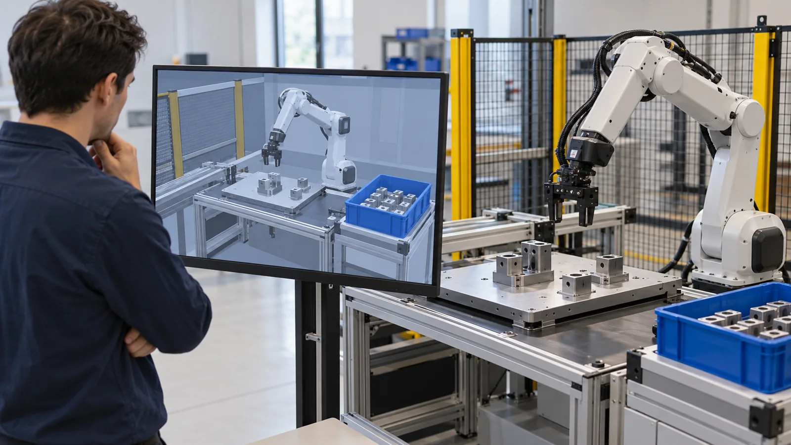
Doing all of a robot’s training and design checks on the real machine takes time and money. So simulators that reproduce robots and their surroundings inside a computer are used. The names MuJoCo, Isaac Sim and Gazebo are familiar, but knowing “what is calculated and what is left out” and “where it departs from the real machine” changes how you read the results. Using analogies a materials engineer can relate to, this article checks, with official documentation and small calculations of our own, what a physics engine does in one step, how the time step relates to the stiffness of contacts, synthetic data, and how material properties such as friction create the gap with the real machine. The second half sorts out what the term “digital twin” means and where it stops. We do not rank particular simulators.
- What robot simulation and digital twins are (the short version)
- What simulation is used for
- What a physics engine does in one step
- Seeing it in numbers — time step and contact stiffness
- The main simulators — reading the official descriptions
- Synthetic data — making “teaching material” by computer
- The gap to the real machine — measuring material properties is the key
- What a digital twin is — meaning and limits
- Limits, and what could not be confirmed / summary
- How to read the yardsticks and standards
- Glossary
- References
- Claim-to-source audit
Sourced = stated in published material (link given)
Our calculation = a figure this article derived, with the assumptions spelled out
Not yet confirmed = a plan, draft or work in progress that is not settled
Interpretations are marked separately as Commentary. Inference is shown in bold.
The numerical examples in Chapters 4 and 7 are calculations from values we assumed (a mass of 0.5 kg, spring constants, friction coefficients and so on). They are not the performance of any real robot, material or simulator. The speed and accuracy of simulators are the developers’ own statements and not a like-for-like comparison. Words such as “fastest” and “high fidelity” are treated as the developers’ claims. For standards (ISO) we confirmed only number, title and stage and did not read the text. We do not compare specific products or companies.
1. What robot simulation and digital twins are (the short version)
- A simulator is a “copy of the real machine”: you enter values such as shape, mass, friction and stiffness, and it solves the equations of physics a little at a time, one time step after another, to reproduce the motion of robots and objects inside a computer. It is useful, but what you did not enter is not reproduced. Contact (things touching) is a particularly hard partSourced[Ref. 2]
- There is a speed-versus-accuracy trade-off in the calculation: a larger time step is faster but less stable. In our calculation the same spring, depending on step size and integration method, diverged in some cases and in others was numerically damped awayOur calculation. The stiffer the contact material, the smaller the step needed
- A digital twin is not the same as a simulator: a digital twin is described as a digital counterpart that exchanges data two ways with the real object and is updated by itSourced[Ref. 21]. It is distinguished from a one-way “shadow” and from a “model” built by people, and it has been pointed out that the term has no common understanding yet [Ref. 20]
In this series’ shared picture, a robot is a combination of “sense (sensors), think (control and intelligence) and act (actuators)”. A simulator runs these three inside a computer so that you can try things without using the real machine. How objects move is set by the law that a force produces acceleration. A simulator solves it over very short intervals (time steps) and updates position and speed a little at a time (like drawing a flip-book one frame at a time; the limit of the analogy: nothing is calculated between the frames).
Our article on imitation and reinforcement learning covers learning in simulation and sim2real from the learning side, and our article on world models and embodied AI sorts out the causes of the reality gap. This article is limited to the simulator itself (what is being calculated) and sorting out the term “digital twin”. Our article on robot foundation models and VLA covers simulated benchmarks, our article on teleoperation and data collection covers collecting data on real machines, and our materials-informatics series covers digital twins in materials (multiscale simulation).
A simulator’s results are decided by “how correct the values you put in are” and “the calculation settings”. The gap to the real machine shrinks when you measure and correct material properties such as friction and stiffness. A simulation built from values nobody measured is a well-made imaginary picture.
2. What simulation is used for
There are four main uses. All of them start from the fact that “doing it on the real thing is heavy in time, cost and safety”.
| Use | What is done | Examples (papers and documents) | Notes (commentary) |
|---|---|---|---|
| Learning a policy | Trial and error with many virtual robots to build a policy | Walking of a quadruped learned in under four minutes on flat terrain and twenty minutes on uneven terrain with GPU parallelism [Ref. 9] | A gap to reality remains (Chapter 7) |
| Evaluating policies and designs | Check motions and design proposals before using the real machine | SIMPLER consists of simulation environments paired with real-robot policy evaluation, reporting strong correlation under particular set-ups [Ref. 19] | Generalisation to other set-ups is not guaranteed |
| Generating synthetic data | Make large amounts of training images or demonstrations by computer | Over 50,000 demonstrations synthesised from about 200 human demonstrations (MimicGen) [Ref. 17] | How to mix with real data matters (Chapter 6) |
| Digital twins | Link to the real machine and use it to grasp state, predict and decide | The framework for manufacturing, ISO 23247 [Ref. 22] | Meaning and limits of the term (Chapter 8) |
Each example is a report by its developers or authors; conditions differ, so we do not compare the numbers. The “Notes” column is this article’s arrangement (commentary).
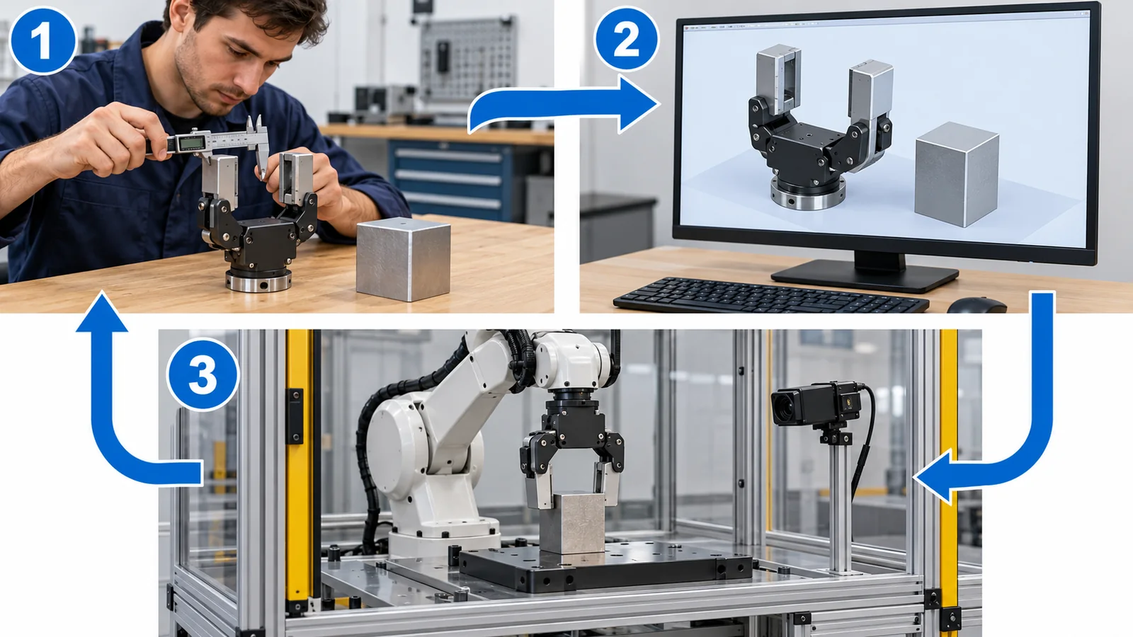
Original SVG, detailed explanation and sources
Original SVG reference: Conceptual diagram (vector drawing). An arrangement of the cycle: measure the real machine and build a model, learn, evaluate and design in a simulator, try the result on the machine, and feed the gap back to the model. Some studies measure the gap to adjust the randomisation distribution [Ref. 15]. It is not the architecture of any particular software.
3. What a physics engine does in one step
The part of a simulator that computes forces, contacts and motion is called the physics engine. One step goes: (1) from the current state (positions and velocities), (2) find what is touching (contact), (3) compute contact forces, friction and joint forces, (4) advance by the time step dt, and (5) obtain the new state. This is repeated over and over.
(1) The time step: a tug of war between “speed” and “stability”
The official MuJoCo documentation gives the default time step as 0.002 s and describes it as the single most important value for the speed-accuracy trade-off. Smaller values raise accuracy and stability but need more computation to advance the same time [Ref. 3]Sourced. To run in real time, that means calculating one second of motion in 500 steps (the inverse of 0.002 s)Our calculation.
(2) Contact: treated as “soft”
When objects touch, even hard materials in reality deform slightly and transmit force. The official MuJoCo documentation says that all physical materials deform somewhat and that the contacting parts of robots are often designed to be soft, and explains that contact is treated with a “soft contact” model that allows slight penetration. Constraint forces are defined as the solution of a convex optimisation problem. The default friction cone is pyramidal [Ref. 2]Sourced.
Real contact is a complex phenomenon set by surface roughness, minute deformation, contamination and temperature. A simulator approximates it with a handful of parameters (spring stiffness, damping, friction coefficient and so on). So where the parameters do not match the real material, or where the approximation does not hold (cloth, liquids, powders), the results drift (commentary).
4. Seeing it in numbers — time step and contact stiffness
Why does the time step decide stability? Let us check with a spring. A mass of 0.5 kg is supported by a spring of 10⁵ N/m (the larger the number, the stiffer the spring) and starts pushed in by 1 mm (an assumption). This is a simplified example of a “stiff contact”. We calculated this oscillation for 0.2 s, varying the time step and the integration method.
The results are as follows (Our calculation).
- Explicit Euler (1 ms): the energy grows to about 7 x 10¹⁵ times its start and the calculation diverges. It is a very simple method, but not suited to oscillating systems
- Semi-implicit Euler (1 ms): the energy stays within about 1.3 times the start, nearly conserved. MuJoCo’s default integrator is this semi-implicit Euler method [Ref. 3]
- Semi-implicit Euler (4 ms): close to the stability limit (ω x dt < 2; here about 1.79) and wobbles up to about 9.5 times
- Semi-implicit Euler (5 ms): ω x dt is about 2.24, beyond the limit, and diverges to about 10³⁴ times
- Implicit Euler (5 ms): it does not diverge, but the energy vanishes artificially (in a system that should keep oscillating). Read it as having dulled the motion for the sake of stability
Our calculation. Assumed mass 0.5 kg, spring constant 10⁵ N/m, initial displacement 1 mm, no damping. Natural angular frequency ω = √(k/m) = about 447 rad/s (period about 14 ms). Not values for any real material or simulator.
The stiffer the contact, the smaller the time step needed
From the condition that semi-implicit Euler stays bounded, ω x dt < 2, the limit of dt is 2√(m/k). Here is the limit for the same mass of 0.5 kg as the contact stiffness k changes (Our calculation).
| Contact spring constant k (N/m, assumed) | Limit of dt (2√(m/k)) | Can 0.002 s (MuJoCo’s default) be used? |
|---|---|---|
| 10⁴ (soft) | about 14.1 ms | Yes (one-seventh of the limit) |
| 10⁵ | about 4.5 ms | Yes |
| 10⁶ | about 1.4 ms | No (above the limit) |
| 10⁷ (stiff) | about 0.45 ms | No (4.5 times the limit) |
Our calculation. The spring constants are assumed values, not those of any particular material or device. Real physics engines treat contacts softly, and the stability condition depends on settings [Ref. 2].
In the table, when the spring constant becomes 100 times larger, the largest time step that can be calculated stably becomes one-tenth. In other words, if you try to calculate a hard contact such as metal on metal exactly as it is in reality, the time step has to be made very small. That robot simulators treat contact as “soft, allowing slight penetration” [Ref. 2] is not only a way of leaving out physics but also a device for making the calculation stable and fast (commentary).
Seen with a materials eye, the “stiffness” and “damping” you enter connect to the elastic modulus and loss of the rubber on a real fingertip and to the surface state of the workpiece. Conversely, softening the fingertip rubber makes contact more stable and easier to grasp in reality too, but a trade-off with positional accuracy and durability appears (this is this article’s general view, not a measurement on any specific device).
5. The main simulators — reading the official descriptions
We sort representative simulators used in robotics by their official descriptions. We do not rank them. The “suited to” column is this article’s arrangement.
| Name (source) | Official or paper description | Licence and release | Suited to (commentary) | Note |
|---|---|---|---|---|
| MuJoCo [Ref. 1, 2] | Stands for Multi-Joint dynamics with Contact. A general-purpose physics engine for robotics, biomechanics, machine learning and more. Acquired by Google DeepMind in October 2021 and open-sourced in May 2022 | Apache-2.0 [Ref. 4] | Control and learning with many contacts | Contact is a soft-contact model (Chapter 3) |
| MuJoCo Playground [Ref. 5] | An open-source framework on MJX. Policies can be trained in minutes on a single GPU. Described as allowing zero-shot sim-to-real on quadrupeds, humanoids, hands and arms | Open source (as stated in the paper) | Training on the GPU and sim2real | Speed and success are the developers’ description |
| Isaac Sim / Isaac Lab [Ref. 6, 7] | Imports URDF, MJCF, USD and more and simulates with PhysX or Newton. Synthetic data generation (Replicator) and ROS 2. Isaac Lab integrates GPU-parallel physics, photorealistic rendering, actuator models, sensors, data collection and domain randomisation | Apache 2.0 (as stated in the official documentation) | Learning that uses photorealistic rendering; synthetic data | Needs computing (GPU) resources |
| Gazebo [Ref. 10, 11] | Presented as an open-source multi-robot simulator; the current repository is gz-sim | Apache-2.0 | System-level checks of a whole robot (often combined with ROS) | Designed differently from large-scale parallel learning platforms (commentary) |
| ManiSkill3 [Ref. 12] | GPU-parallel simulation and rendering. Described by its developers as 10 to 1000 times faster than other platforms, with over 30,000 FPS in benchmark environments | Open source (as stated in the paper) | Parallel learning of manipulation tasks | “Fastest” is the developers’ claim |
The table is Sourced from the descriptions in official documentation and papers (licences were checked through GitHub’s public API or the official documentation, 25 October 2026). The “suited to” column is this article’s arrangement (commentary). There are many other simulators, but we limit ourselves to what we could confirm.
GPU parallelism: orders of magnitude more trials in the same time
The Isaac Gym paper reports that running physics simulation and policy training together on the GPU gave a speed-up of two to three orders of magnitude over conventional simulators running on the CPU [Ref. 8]Sourced. Rudin et al. report that with this approach an ANYmal walking policy could be learned on uneven terrain in 20 minutes [Ref. 9]. Running many environments at once makes possible a quantity of trials that is impossible on real machines. These speed figures, however, are for the tasks and computers chosen by their developers and authors (commentary).
6. Synthetic data — making “teaching material” by computer
A simulator can produce not only motion but also training data. The main ways of using it are as follows.
- Images with varied appearance: Tobin et al. report that a real-world object detector accurate to 1.5 cm could be learned from simulator images with only non-realistic random textures [Ref. 13]. Isaac Sim describes a framework for synthetic data generation (Replicator) [Ref. 6]Sourced
- Many demonstrations from a few: MimicGen converted about 200 human demonstrations to fit new scenes, objects and robot arms and automatically produced over 50,000 demonstrations on 18 tasks (about 250 times as many). It reports that imitation learning on this synthetic data gave strong performance on long-horizon and high-precision tasks, comparing favourably with collecting additional human demonstrations [Ref. 17]SourcedOur calculation (250 times = 50,000 / 200)
- Large-scale environments: RoboCasa is a large-scale simulation centred on kitchens, with thousands of 3D assets in over 150 object categories, and reports a trend of improving performance with the amount of synthetic data [Ref. 18]Sourced
In fact: synthetic data rest on the physics and appearance inside the computer, so phenomena you did not put in are absent. Many papers combine synthetic data with real data or confirm results on real machines. It is not certain that “synthetic data alone can solve a real-world task”. The amount and quality of synthetic data and the ratio to real data must be checked for each task (commentary).
7. The gap to the real machine — measuring material properties is the key
The gap between simulation and the real machine (the reality gap) has many causes. Here we focus on material properties that can be shrunk by measurement. The overall arrangement of the causes is in Chapter 4 of our article on world models and embodied AI.
| Cause of the gap | Simulator side (model) | Real side | Examples of how to measure or respond (commentary) |
|---|---|---|---|
| Friction | Approximated by one friction coefficient (or a friction cone) | Changes with surface roughness, contamination, humidity, temperature and contact force | Measure the angle at which a sample slides on a tilted plate. Measure the range and randomise it [Ref. 14] |
| Contact stiffness and damping | A few parameters of spring and damping | Elastic modulus, loss and surface state of the material | Measure by indentation tests and the like. Balance with the time step (Chapter 4) |
| Motors and gears | An actuator model (force, speed and lag characteristics) [Ref. 7] | Backlash and friction of gears and their change with temperature | Measure the real machine’s response and fix the model values (system identification) |
| Sensors | Ideal values, or a noise model | Delay, noise and calibration drift | Compare with recordings from the real machine |
| Deformable objects | Approximated as rigid, or a simple model | Complex deformation of cloth, cables, powders and liquids | A hard area to reproduce. Evaluate on the real machine |
The table is this article’s arrangement (commentary), and the “how to measure or respond” entries are general examples. That Isaac Lab provides actuator models is stated in its paper, and that friction is randomised is stated in the OpenAI paper.
A calculation of how a friction error affects the grip force
Let us see the size of a friction-coefficient error with a simple example. To lift an object pinched between two fingers without slipping, the force N each finger needs follows from the condition that the friction force 2μN of the two fingers supports the object’s weight mg: N = mg / (2μ) (a formula with no safety factor). Take an object of 0.5 kg whose friction coefficient is 0.5 in the simulator and 0.3 on the real machine.
- Simulator (μ = 0.5): N = 0.5 x 9.81 / (2 x 0.5) = about 4.9 N
- Real machine (μ = 0.3): N = 0.5 x 9.81 / (2 x 0.3) = about 8.2 N (about 1.67 times the simulator’s)
- So a policy that learned in simulation that “about 5 N is enough” may drop the object on a real machine whose friction coefficient is 0.3Our calculation
Our calculation. Mass 0.5 kg, gravitational acceleration 9.81 m/s², friction coefficients 0.5 and 0.3 are illustrative assumptions, not values of real materials. Real grasping also involves finger shape, contact area and dynamic forces; this is a simplification.
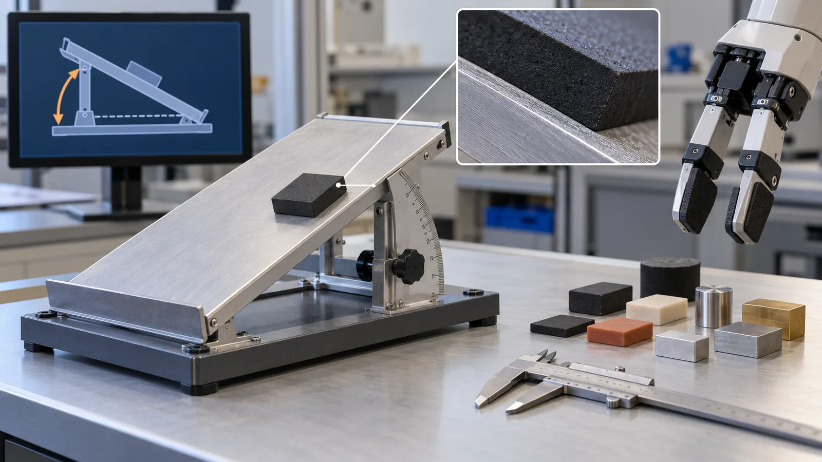
A friction coefficient depends not only on the kind of material but on surface state (roughness, contamination, oil, humidity) and conditions (load, speed, temperature). Before entering a catalogue value or a value from a paper as it is, it is worth measuring it for your own fingertip and object pair. If you measure the angle at which a sample starts to slide on a tilted plate, the friction coefficient is easily estimated as tan θ (μ = tanθ; 0.5 is about 26.6° and 0.3 about 16.7°)Our calculation.
Furthermore, giving not a single value but the spread of the measurements becomes the basis for the range of domain randomisation [Ref. 14]. A method of collecting a few real-machine roll-outs and correcting the randomisation distribution has also been reported [Ref. 15]Sourced. This is one of the places where materials knowledge helps most.
The gap in evaluation: a simulated score is no substitute for a real-machine score
SIMPLER built simulation environments paired with real-robot policy evaluation and reports that, in paired evaluations, policy performance correlated strongly between the two and that behaviours such as sensitivity to distribution shift were also reflected. This is a result for particular robot set-ups and does not necessarily hold for all [Ref. 19]Sourced. An overview of sim2real methods is organised in the survey by Zhao et al. [Ref. 16].
8. What a digital twin is — meaning and limits
“Digital twin” is a widely used term, but its meaning varies. Kritzinger et al. divide the manufacturing literature by level of integration into digital model, digital shadow and digital twin, and state that there is no common understanding of the term and that papers at the most advanced level, the digital twin, are scarce [Ref. 20]Sourced. A report of the US National Academies of Sciences, Engineering, and Medicine describes a digital twin as something that couples a computational model with a physical counterpart and is updated through bidirectional data flows [Ref. 21]Sourced.
An international standard for manufacturing
In manufacturing, the ISO 23247 series sets out a framework for digital twins. ISO 23247-1:2021 covers an overview and general principles of the digital-twin framework for manufacturing (terms and requirements), and ISO 23247-2:2021 a reference architecture (a reference model from domain and entity viewpoints, and a functional view) [Ref. 22, 23]Sourced. We did not read the text, which is paid, and it is not a standard specific to simulators for robot learning.
Limits: why a digital twin is not all-powerful
- Scope of the model: a twin reproduces only the phenomena put into it. Simplifications of friction or deformation lead to wrong decisions (Chapters 3 and 7)
- Quality and updating of data: if the sensor data representing the real object’s state are delayed, off or missing, the twin drifts away from the real object (commentary)
- Degradation of the real object: wear, contamination and ageing change the real object, so the twin’s values must keep being updated (this is this article’s general view)
- How the word is used: something called a “digital twin” may in fact be a model built by people or a one-way shadow. Check whether data flow both ways and whether predictions and decisions return to operation
In fact: a twin’s accuracy is set by the material properties entered and by the quality of the sensor data. If the real object’s state departs from the twin’s assumptions, the results drift. For important decisions you need confirmation on the real object, or monitoring of the difference between the twin’s prediction and measurement. A twin is not “a replacement for the real thing” but “a tool used in a pair with the real thing” (commentary).
9. Limits, and what could not be confirmed / summary
(1) Comparing simulators
The speed and accuracy of each simulator are the developers’ or authors’ statements and not a like-for-like comparison. We did not confirm independent third-party comparisons. Words such as “fastest” and “high fidelity” are treated as developers’ claims, and we do not rank them.
(2) Calculations from assumed values
The numbers in Chapters 4 and 7 are arithmetic on assumptions we made (mass, spring constant, friction coefficient), not values for real materials, devices or simulators. The stability condition ω x dt < 2 is that of semi-implicit Euler for a simple spring; the stability conditions of real engines are more complicated.
(3) The text of standards
We did not read the text of ISO 23247. We could not confirm an international standard that defines the fidelity of robot simulators.
(4) The text of Kritzinger et al.
The publisher’s page refused automated access, so we cite only within the bibliographic data and abstract. We did not check the text for the detailed definitions of the three levels.
(5) What we did not cover
Multiscale simulation of materials is in our materials-informatics series and the details on the learning side in our article on imitation and reinforcement learning. We do not cover market size or prices.
- A simulator is a “copy of the real machine” that solves the equations of physics one time step at a time. Results change with step size and integration method, and stiffer contacts need smaller stepsSourcedOur calculation
- The gap to the real machine shrinks by measuring material properties such as friction and stiffness. We calculated an example in which friction coefficients of 0.5 and 0.3 change the required grip force by about 1.67 timesOur calculation
- A digital twin is described as something that exchanges data two ways with the real object and is updated by it, but there is no common understanding of the term; read it distinguished from simulators and one-way shadowsSourced
10. How to read the yardsticks and standards
The basic yardstick for a simulator is how well it corresponds to the real machine (correlation, or differences in results). Speed (steps per second), stability (does it diverge?) and reproducibility (does it give the same result?) matter too. For digital twins there is a framework standard for manufacturing (checked 25 October 2026).
| Item evaluated | Representative tests and benchmarks (name, source) | Standards, rules and guidance (ISO and others) | Notes on reading |
|---|---|---|---|
| Correspondence between simulation and real machine | SIMPLER (strong correlation in paired evaluation; particular robot set-ups) [Ref. 19]Sourced | We could not confirm an international standard defining the fidelity of robot simulators | Generalisation to other robots and tasks is not guaranteed |
| Speed of calculation | Developers’ statements (Isaac Gym: two to three orders of magnitude faster [Ref. 8]; ManiSkill3: over 30,000 FPS at most [Ref. 12])Sourced | Could not be confirmed | Tasks, computers and settings differ. Developers’ claims |
| Stability of calculation (step and integrator) | Our calculation (ω x dt < 2). MuJoCo’s official documentation (default 0.002 s) [Ref. 3]Our calculationSourced | Could not be confirmed | The stability condition differs by engine and model |
| Effect of synthetic data | MimicGen (about 200 to over 50,000 demonstrations) [Ref. 17], RoboCasa (trend with amount of synthetic data) [Ref. 18]Sourced | Could not be confirmed | Results change with the mix with real data and the evaluation tasks |
| Digital twins in manufacturing | — (a framework, not a benchmark) | ISO 23247-1:2021 (overview and general principles) and ISO 23247-2:2021 (reference architecture) [Ref. 22, 23]Sourced | A framework for manufacturing, not specific to simulators for robot learning. The text is paid |
The arrangement of the table is Our calculation (organising). Numbers, titles, dates and stages of ISO standards were checked on the official ISO pages (25 October 2026). The text of the standards is paid, so we stay with titles and scope.
Notes on reading (for materials engineers)
- Simulation results follow the correctness of the values entered: check whether friction, stiffness and damping are measured or provisional values, and match the measurement conditions (load, surface state, temperature)
- A developer’s speed and accuracy are the developer’s claims: tasks and computers differ, so do not rank by lining up the numbers
- Is a standard a requirement or a framework? ISO 23247 is a framework for digital twins in manufacturing and does not guarantee the fidelity of a simulator for robot learning
- Watch the words “digital twin”: check whether data flow in both directions and whether predictions and decisions return to operation
11. Glossary
- Simulator
- Software that reproduces the motion of robots and environments inside a computer by calculating physical laws.
- Physics engine
- The part of a simulator that computes forces, contacts and motion.
- Time step
- The length of time advanced in one calculation step.
- Numerical integration
- Solving the equations of motion bit by bit, one time step at a time.
- Semi-implicit Euler method
- A common integrator that updates velocity first and then position.
- Rigid body
- An object treated as not deforming.
- Contact
- Objects touching and exchanging force.
- Soft contact
- A model that treats contact as “soft”, allowing slight penetration.
- Friction cone
- A cone representing the range of contact forces that can be transmitted without slipping.
- Stiffness (spring constant)
- Resistance to deformation, expressed in N/m.
- System identification
- Measuring a real machine’s response to determine the model’s values (mass, friction and so on).
- Domain randomisation
- Training with the simulator’s appearance and physical values varied so that the policy tolerates differences.
- Sim2real / reality gap
- Moving what was learned in simulation to the real machine / the difference between the two.
- Parallel simulation
- Computing many environments at once (for example on a GPU) to collect training data quickly.
- Synthetic data
- Training data made by computer.
- Actuator model
- The force, speed and lag characteristics of motors and gears put into a simulator.
- URDF / MJCF / USD
- File formats for describing robots and scenes (used with ROS, MuJoCo and OpenUSD respectively).
- Digital model
- A digital copy of a real object built by people entering values, with no automatic data exchange with it.
- Digital shadow
- A digital copy updated automatically by data flowing from the real machine (one way).
- Digital twin
- A digital counterpart that exchanges data two ways with the real object and is used for updating, prediction and decisions.
12. References
- Todorov E., Erez T., Tassa Y. “MuJoCo: A physics engine for model-based control”, IEEE/RSJ IROS 2012, 5026–5033, DOI 10.1109/IROS.2012.6386109 — doi.org/10.1109/IROS.2012.6386109
- Google DeepMind MuJoCo documentation, “Computation” (soft contact model, constraint solver). Checked 25 October 2026 — mujoco.readthedocs.io (computation)
- Google DeepMind MuJoCo documentation, “XML Reference” (option: timestep, integrator). Checked 25 October 2026; values confirmed in the documentation source on GitHub — mujoco.readthedocs.io (XML reference)
- Google DeepMind GitHub repository “google-deepmind/mujoco” (Apache License 2.0). Licence confirmed through GitHub’s public API (25 October 2026) — github.com/google-deepmind/mujoco
- Zakka K. et al. “MuJoCo Playground”, arXiv:2502.08844 (2025) — arxiv.org/abs/2502.08844
- NVIDIA Isaac Sim documentation (overview). Checked 25 October 2026 — docs.isaacsim.omniverse.nvidia.com
- NVIDIA et al. “Isaac Lab: A GPU-Accelerated Simulation Framework for Multi-Modal Robot Learning”, arXiv:2511.04831 (2025) — arxiv.org/abs/2511.04831
- Makoviychuk V. et al. “Isaac Gym: High Performance GPU-Based Physics Simulation For Robot Learning”, arXiv:2108.10470 (2021) — arxiv.org/abs/2108.10470
- Rudin N. et al. “Learning to Walk in Minutes Using Massively Parallel Deep Reinforcement Learning”, arXiv:2109.11978 (2021) — arxiv.org/abs/2109.11978
- Koenig N., Howard A. “Design and use paradigms for Gazebo, an open-source multi-robot simulator”, IEEE/RSJ IROS 2004, 2149–2154, DOI 10.1109/IROS.2004.1389727 — doi.org/10.1109/IROS.2004.1389727
- Gazebo / Open Robotics GitHub repository “gazebosim/gz-sim” (Apache License 2.0). Licence confirmed through GitHub’s public API (25 October 2026) — github.com/gazebosim/gz-sim
- Tao S. et al. “ManiSkill3: GPU Parallelized Robotics Simulation and Rendering for Generalizable Embodied AI”, arXiv:2410.00425 (2024) — arxiv.org/abs/2410.00425
- Tobin J. et al. “Domain Randomization for Transferring Deep Neural Networks from Simulation to the Real World”, arXiv:1703.06907 (2017) — arxiv.org/abs/1703.06907
- OpenAI et al. “Learning Dexterous In-Hand Manipulation”, arXiv:1808.00177 (2018) — arxiv.org/abs/1808.00177
- Chebotar Y. et al. “Closing the Sim-to-Real Loop: Adapting Simulation Randomization with Real World Experience”, arXiv:1810.05687 (2018) — arxiv.org/abs/1810.05687
- Zhao W., Queralta J. P., Westerlund T. “Sim-to-Real Transfer in Deep Reinforcement Learning for Robotics: a Survey”, arXiv:2009.13303 (2020) — arxiv.org/abs/2009.13303
- Mandlekar A. et al. “MimicGen: A Data Generation System for Scalable Robot Learning using Human Demonstrations”, arXiv:2310.17596 (2023) — arxiv.org/abs/2310.17596
- Nasiriany S. et al. “RoboCasa: Large-Scale Simulation of Everyday Tasks for Generalist Robots”, arXiv:2406.02523 (2024) — arxiv.org/abs/2406.02523
- Li X. et al. “Evaluating Real-World Robot Manipulation Policies in Simulation” (SIMPLER), arXiv:2405.05941 (2024) — arxiv.org/abs/2405.05941
- Kritzinger W. et al. “Digital Twin in manufacturing: A categorical literature review and classification”, IFAC-PapersOnLine 51(11), 1016–1022 (2018), DOI 10.1016/j.ifacol.2018.08.474. Bibliographic data and abstract confirmed (via Semantic Scholar); the publisher’s page refused automated access — doi.org/10.1016/j.ifacol.2018.08.474
- National Academies of Sciences, Engineering, and Medicine “Foundational Research Gaps and Future Directions for Digital Twins” (2024), DOI 10.17226/26894. Checked 25 October 2026 — nationalacademies.org/publications/26894
- ISO ISO 23247-1:2021 “Automation systems and integration — Digital twin framework for manufacturing — Part 1: Overview and general principles” (Edition 1, October 2021). Checked 25 October 2026 — iso.org/standard/75066.html
- ISO ISO 23247-2:2021 “Automation systems and integration — Digital twin framework for manufacturing — Part 2: Reference architecture” (Edition 1, October 2021). Checked 25 October 2026 — iso.org/standard/78743.html
13. Claim-to-source audit
| Claim in the text | Basis | Class |
|---|---|---|
| That MuJoCo stands for Multi-Joint dynamics with Contact and is a general-purpose physics engine for robotics, biomechanics, machine learning and more; that Google DeepMind acquired it in October 2021 and open-sourced it in May 2022; that its licence is Apache-2.0 | MuJoCo documentation (overview), GitHub public API, Todorov et al. (title) Reference 1 https://doi.org/10.1109/IROS.2012.6386109 Reference 4 https://github.com/google-deepmind/mujoco | Sourced |
| That MuJoCo’s default time step is 0.002 s and is the most important parameter for the speed-accuracy trade-off; that the default integrator is semi-implicit Euler (with RK4 and implicit options) | MuJoCo documentation (XML Reference, option) Reference 3 https://mujoco.readthedocs.io/en/stable/XMLreference.html | Sourced |
| That MuJoCo treats contact with a soft-contact model allowing slight penetration; the explanation that all physical materials deform somewhat and the contacting parts of robots are often designed to be soft; that the default friction cone is pyramidal; that constraint forces are defined as the solution of a convex optimisation problem | MuJoCo documentation (Computation, Modeling) Reference 2 https://mujoco.readthedocs.io/en/stable/computation/index.html | Sourced |
| The official Isaac Sim documentation: import of URDF, MJCF and USD, simulation with PhysX or Newton, synthetic data generation (Replicator), ROS 2, USD-native, Apache 2.0 | NVIDIA documentation Reference 6 https://docs.isaacsim.omniverse.nvidia.com/latest/index.html | Sourced |
| Isaac Lab: a framework integrating GPU-parallel physics, photorealistic rendering, actuator models, sensor simulation, data collection and domain-randomisation tools; Isaac Gym: physics and policy learning on the GPU, two to three orders of magnitude faster than conventional CPU simulators; Rudin et al.: under four minutes on flat terrain and twenty minutes on uneven terrain | NVIDIA et al. (abstract); Makoviychuk et al.; Rudin et al. Reference 7 https://arxiv.org/abs/2511.04831 Reference 8 https://arxiv.org/abs/2108.10470 Reference 9 https://arxiv.org/abs/2109.11978 | Sourced |
| MuJoCo Playground: an open-source framework on MJX in which policies can be trained in minutes on a single GPU, with zero-shot sim-to-real on quadrupeds, humanoids, hands and arms as described; ManiSkill3: GPU-parallel simulation and rendering described by its developers as 10 to 1000 times faster than other platforms, with over 30,000 FPS | Zakka et al.; Tao et al. (abstracts; developers’ descriptions) Reference 5 https://arxiv.org/abs/2502.08844 Reference 12 https://arxiv.org/abs/2410.00425 | Sourced |
| That Gazebo was presented in a paper as an open-source multi-robot simulator and that the current repository (gz-sim) is under Apache-2.0 | Koenig and Howard (title); GitHub public API Reference 10 https://doi.org/10.1109/IROS.2004.1389727 Reference 11 https://github.com/gazebosim/gz-sim | Sourced |
| Domain randomisation (Tobin et al.); learning with Shadow Hand using randomised friction coefficients and other values (OpenAI); adapting the randomisation distribution with real-world roll-outs (Chebotar et al.); an overview of sim2real methods (the survey by Zhao et al.) | Abstracts of the respective papers Reference 13 https://arxiv.org/abs/1703.06907 Reference 14 https://arxiv.org/abs/1808.00177 Reference 15 https://arxiv.org/abs/1810.05687 Reference 16 https://arxiv.org/abs/2009.13303 | Sourced |
| MimicGen: over 50,000 demonstrations on 18 tasks synthesised from about 200 human demonstrations; RoboCasa: a large-scale kitchen-centred simulation reported to show a scaling trend with synthetic data; SIMPLER: simulation environments paired with real-robot policy evaluation, with strong correlation to the real machine on particular robot set-ups | Mandlekar et al.; Nasiriany et al.; Li et al. (abstracts) Reference 17 https://arxiv.org/abs/2310.17596 Reference 18 https://arxiv.org/abs/2406.02523 Reference 19 https://arxiv.org/abs/2405.05941 | Sourced |
| Classification of digital twins: Kritzinger et al. distinguish digital model, digital shadow and digital twin by level of integration, noting no common understanding of the term and few papers at the digital-twin level; a US National Academies report: a computational model coupled with a physical counterpart and updated through bidirectional data flows | Kritzinger et al. (abstract); the Academies report (publication page) Reference 20 https://doi.org/10.1016/j.ifacol.2018.08.474 Reference 21 https://www.nationalacademies.org/publications/26894 | Sourced |
| The numbers, titles, publication (October 2021) and scope of ISO 23247-1:2021 (digital twin framework for manufacturing, overview and general principles) and ISO 23247-2:2021 (reference architecture) | ISO pages Reference 22 https://www.iso.org/standard/75066.html Reference 23 https://www.iso.org/standard/78743.html | Sourced |
| The energy curves for time step and integrator in Figure 4, the time-step limits in Figure 5 (2 sqrt(m/k): 4.5 ms, 1.4 ms and so on), the grip forces in Figure 6 (mg / 2 mu: 4.9 N, 8.2 N) and the factor 1.67, and the factor of 250 for MimicGen (50,000 / 200) | Our calculation (Python, NumPy; the mass of 0.5 kg, spring constant of 10⁵ N/m and so on are assumptions; stability condition w dt < 2 of semi-implicit Euler). Not values for real materials or devices | Our calculation |
| The readings that a simulator is a copy of the real machine that must keep being corrected by measurement, that friction and stiffness values enter only if measured, that a digital twin is not the same as a simulator, and that one should not rely on synthetic data alone | This article’s commentary based on the published material; not views stated by the institutions | Commentary |
| An international standard defining the fidelity of robot simulators, a standard specific to digital twins in robotics, independent comparisons of the superiority or speed of simulators, and measured friction values for real machines | Not included because they could not be confirmed from primary sources within this article’s research (commentary) | Commentary |
| That Figures 1 and 7 are frames for AI-generated images, Figures 2, 3 and 8 are explanatory concept diagrams, and Figures 4, 5 and 6 contain our calculations | This article’s own note | Commentary |
Last updated: 25 October 2026 / Sources are limited to primary material (arXiv papers, official documentation, public GitHub information, the official ISO pages and a report of the US National Academies). We could not read the text of the ISO standards or of the paper by Kritzinger et al. The numerical examples are calculations from values we assumed and are not the performance of any real material, device or simulator. We could not confirm, and so do not state, an international standard defining the fidelity of robot simulators, independent comparisons of simulators, or measured friction values for real machines. Figures 1 and 7 are ImageGen-generated conceptual illustrations; the other figures are explanatory concept diagrams or figures containing our calculations.