SLAM and Localization Explained

TECHNOLOGY EXPLAINER

SLAM and Localization
– Knowing “where am I” while building the map

To move around on its own, a robot or drone has to know where it is. Outdoors it can use GPS, but indoors or under a bridge GPS fails. The answer is SLAM (pronounced “slam”): estimate your own position while building a map of your surroundings, by combining sensors such as cameras, LiDAR, IMUs and GNSS. This article explains, with figures and numerical examples, what each sensor is good at, why errors pile up (drift), and how returning to a known place lets the system correct itself (loop closure). The second half covers how drones and ground robots use SLAM differently, and how materials and mounting affect SLAM accuracy.

Sources: survey articles and papers (IEEE Transactions on Robotics and others), GPS.gov, PX4 documentation, official dataset and benchmark pages, a DJI specification, official ISO pages / calculations are our own / checked 25 October 2026

Fig. 1. Concept illustration generated with ImageGen. Concept diagram (AI-generated image). An image of a drone and a ground robot moving in a warehouse while building a map with cameras and sensors. These are not real vehicles, products or facilities. Not an actual product, facility or measurement. Cutaways, colours and arrows explain the concept; proportions are illustrative.

Contents

What is SLAM? (the short version)
Four sensors: camera, LiDAR, IMU, GNSS
Adding up motion makes errors pile up (drift)
How SLAM works: front end and back end
Loop closure: fix everything when you return
Orders of position error
Drone or ground robot: how use differs
Materials and mounting decide SLAM accuracy
How to read the yardsticks and standards
Limits, what could not be confirmed, and summary
Glossary
References (primary sources)
Claim-to-source audit

How this article labels things

Sourced = stated in a published source (linked)
Our calculation = our own calculation from published numbers or stated assumptions
Not yet confirmed = experimental features, drafts and other things not settled
Inference is shown in bold. Readings that have no source are marked “commentary”.

How to read the numbers in this article

The accuracy figures in papers and datasets were measured on a specific dataset under specific conditions. They are not accuracy in the field. Manufacturer numbers are “company’s stated values”. Position error means different things in different places – absolute position error, mean trajectory error, ratio to distance travelled – so we do not rank them against each other. The curves in Figs. 4, 5 and 9 come from our own calculation with stated assumptions, not from a specific product or method. We give no individual advice on safety or regulation.

1. What is SLAM? (the short version)

SLAM = estimating your position while building a map of your surroundings. The name stands for Simultaneous Localization and Mapping. A survey paper defines it as building a model (map) of the environment and estimating the state of the robot moving inside it, at the same time [Reference 1] Sourced
The difficulty is chicken-and-egg: with a map you can find your position, and with your position you can build a map. At the start you have neither, so you estimate both together (analogy: walking through an unknown town, drawing the map as you go and using it to check where you are. Where it fails: in practice sensor errors add up at every step)
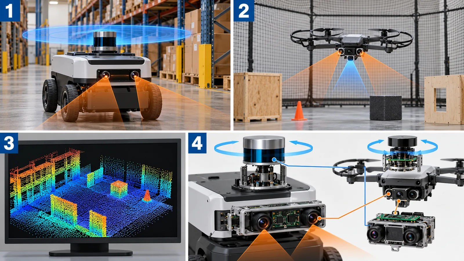
One sensor is not enough: camera, LiDAR, IMU and GNSS each have strengths and weaknesses. On drones the camera-plus-IMU combination (VIO) is widely used [Reference 3]; on ground transport robots SLAM with a 2D LiDAR is the standard [Reference 8] (Fig. 8)

Before you read on

This series describes a robot as a combination of “sensing, thinking (control and intelligence), and moving (actuators)”. This article connects sensing and thinking: own position and the map. Pose means position (x, y, height) plus attitude (heading): six quantities in all (six degrees of freedom). Odometry means estimating position by adding up small motions.

Place in the series: how LiDAR itself works is in the “LiDAR” article, maps and localization for cars in “Autonomous Driving and AI”, drone positioning and collision avoidance in “Drone Communication, Positioning and Collision Avoidance”, on-board computing in “Edge AI and On-Device AI”, and camera recognition in “Robot Vision and Perception”. To avoid overlap, this article keeps to the idea of SLAM and how its use differs.

Fig. 2 Concept diagram (vector drawing). The overall flow of SLAM (top) and an example of pose-graph correction (bottom). A pose graph links points (robot poses) with lines (motion constraints). It is a diagram for explanation, not the structure of any real system [References 1, 2, 4].

2. Four sensors: camera, LiDAR, IMU, GNSS

Here are the four sensors used in SLAM, by what they measure and what they do well and poorly (Fig. 3).

Fig. 3 Concept diagram (vector drawing). Our arrangement of the characteristics of the four sensors. For the basis of each item see the sources under the figure and the text. It does not show the performance of any product [References 4, 9, 10, 14].

GNSS: gives absolute position, but depends on the place

GNSS (satellite positioning such as GPS) gives absolute position on Earth directly. Its strength is that error does not pile up over time. But accuracy varies a lot with conditions. GPS.gov states that smartphone GPS is typically accurate to within a 4.9 m radius under open sky, and that accuracy gets worse near buildings, bridges and trees [Reference 10] Sourced. For high-quality single-frequency GPS receivers, FAA data put the horizontal error at 1.82 m or less with 95% probability [Reference 10] Sourced. It also says that dual-frequency receivers and augmentation systems (such as RTK) can bring this to within a few centimetres in real time [Reference 10] Sourced.

Common misconception: “GPS is accurate to 2 metres”

GPS.gov explains that the commitment of 2.0 m or less (95%) is for the ranging error of the signal in space (URE), not for the user’s position accuracy [Reference 10] Sourced. User accuracy depends on satellite geometry, how the signal is blocked, the atmosphere and the receiver [Reference 10]. The correct picture: “the quality of the signal” and “the accuracy of the position in your hand” are different, and the latter depends on environment and receiver.

3. Adding up motion makes errors pile up (drift)

An IMU (inertial measurement unit) measures acceleration and rotation rate at a high rate. Integrating acceleration twice gives position, so in theory an IMU alone can track position (inertial navigation). But Woodman’s technical report shows that a constant acceleration error (bias) e, integrated twice, gives a position error of e x t^2 / 2, growing with the square of time [Reference 9] Sourced.

Check with numbers. With an acceleration error of 0.01 m/s2 (assumed), the position error after 60 s is 0.01 x 3600 / 2 = 18 m Our calculation. And if the attitude (tilt) of the vehicle is wrong by 0.1 degrees, the gravity component 9.81 x sin 0.1 deg = 0.0171 m/s2 leaks in as an acceleration error. After 60 s that is about 31 m Our calculation (Fig. 4). Woodman reports that with a low-cost IMU of 2007 (Xsens MTx) the position error exceeded 150 m on average in 60 s [Reference 9] Sourced. The report points out that attitude error (gyro noise) is the main cause of position error [Reference 9] Sourced.

Fig. 4 Chart with our calculation (vector drawing). How position error grows when position is tracked with an IMU alone. The formula is from Woodman [Reference 9]; the error sizes (0.01 m/s2, 0.1 degrees) are our assumptions. The red dot is a 2007 experimental value, not the performance of an IMU today.

A sticking point: why does it grow with the square?

An acceleration error first becomes a velocity error (proportional to time), and that velocity error becomes a position error (again proportional to time). Errors feed on errors, so the growth is quadratic. It is like walking with your eyes closed and drifting slightly off course at every step: the farther you go, the larger the offset (where the analogy fails: IMU error also changes with temperature and vibration).

SLAM holds this problem down with other sensors. Cameras and LiDAR can measure the positional relation to the surrounding scene, so they can correct IMU error. For VIO (Visual-Inertial Odometry), which combines a camera and an IMU, Scaramuzza and Zhang write that it is the only viable way to achieve accurate state estimation without relying on GPS or LiDAR odometry, and that cameras and IMUs are cheap and found on all of today’s aerial robots [Reference 3] Sourced.

4. How SLAM works: front end and back end

SLAM has two main parts (Fig. 2, top). The front end quickly estimates small motions from sensor data (odometry). The back end takes the path and map so far and optimizes them together so that everything is consistent (commentary: the survey [Reference 1] treats this “front end and back end” structure as the standard formulation). A common back end uses a pose graph: robot poses are points, relations between them are lines (constraints), and the optimizer searches for the arrangement with the smallest overall error.

Representative methods (as stated in their abstracts)

Method	Main sensors	Features (as described in the paper or survey)
ORB-SLAM3 (Campos et al., 2021) [2]	Camera (mono, stereo, RGB-D), IMU	The first system able to handle visual, visual-inertial and multi-map SLAM. Reports a mean accuracy of 3.6 cm on EuRoC drone data with stereo-inertial, and 9 mm on handheld TUM-VI Sourced
VINS-Mono (Qin et al., 2018) [4]	Monocular camera, IMU	One camera plus a cheap IMU is the minimum setup for metric 6-DOF estimation. With no direct distance measurement, initialization, extrinsic calibration and optimization are the challenges. Has loop detection and 4-DOF pose-graph optimization. Closed-loop autonomous flight on a vehicle Sourced
LIO-SAM (Shan et al., 2020) [5]	LiDAR, IMU	A tightly coupled LiDAR-inertial odometry built on a factor graph. Integrates the IMU to correct distortion of the LiDAR point cloud. Loop closure and other measurements can be added as constraints Sourced
FAST-LIO2 (Xu et al., 2022) [6]	LiDAR, IMU	An iterated Kalman filter registers raw points directly to the map with no feature extraction. The map is kept in an incremental k-d tree (ikd-Tree). Reported more accurate and less computationally heavy than other methods on 19 sequences Sourced
LOAM (Zhang and Singh, 2014) [7]	LiDAR	Real-time LiDAR odometry and mapping (only title and bibliography checked)
Cartographer (Hess et al., 2016) [8]	2D LiDAR	A backpack mapping device with real-time mapping at 5 cm resolution and loop closure. Uses branch-and-bound for loop closure Sourced

Each row is a fact Sourced from the abstract or description in the paper or survey (LOAM: title only). The arrangement of the table is Our calculation. We do not argue which method is better here.

5. Loop closure: fix everything when you return

Front-end error grows as you travel (drift). Drift is usually expressed as a ratio to the distance travelled. The KITTI odometry evaluation measures, over segments of 100 to 800 m, translation error in [%] and rotation error in [deg/m] and ranks methods by the average [Reference 18] Sourced. The public ranking lists, as one LiDAR method, a translation error of 0.61% (checked 25 October 2026) [Reference 18] Sourced. 0.61% means about 6.1 m after 1 km and about 0.61 m after 100 m Our calculation.

Fig. 5 Chart with our calculation (vector drawing). Position error against distance travelled. The grey dashed line is 1.0% (our assumption), blue is one entry of the public KITTI ranking (0.61%), and red and green show a case where the robot returns to the same place at 800 m and loop closure corrects the error (the corrected value is illustrative).

This is where loop closure helps. When the robot notices it has come back to a place it visited before (place recognition), it can add the constraint “these two poses are at the same place” to the pose graph. The back end then optimizes everything and redistributes the accumulated error over the whole path (Fig. 2 bottom, Fig. 5). ORB-SLAM3 uses place recognition to start a new map when visual information is too poor and the map is lost, and to merge maps automatically when it returns to a known place [Reference 2] Sourced.

Common misconception: “With SLAM, GPS is not needed”

SLAM estimates relative position, so error builds up little by little. GNSS gives absolute position whose error does not build up. They complement each other and are commonly combined (commentary). For example, PX4 provides a dead-reckoning mode for environments where GNSS is lost for a while (under a bridge, moving from outdoors to indoors, jamming). But it describes the mode as “new and with limited testing on real vehicles” (v1.17), not meant for flight that starts without GNSS at take-off, and requiring another velocity or position sensor [Reference 15] SourcedNot yet confirmed. The correct picture: SLAM and similar methods bridge the time when GNSS is unavailable; they do not make GNSS unnecessary.

Size of the map: orders of memory

Holding a map takes memory. For example, a 100 m x 100 m plane at the 5 cm resolution of Cartographer [Reference 8] as an occupancy grid is 2000 x 2000 = 4.0 x 10^6 cells. At 1 byte per cell (assumed) that is about 4 MB Our calculation. In 3D, 100 m x 100 m x 10 m height in 10 cm voxels is 1000 x 1000 x 100 = 1.0 x 10^8 cells, about 100 MB even at 1 byte per cell Our calculation. A 3D map becomes heavy quickly with resolution and extent. On a drone’s small computer, how the map is held (keep it as a point cloud, thin it out, and so on) is a key design point (commentary).

6. Orders of position error

Let us line up the numbers so far by size of error (Fig. 6). Smartphone GNSS gives several metres, a high-quality single-frequency receiver within 2 m, RTK a few centimetres, and visual-inertial SLAM several centimetres to millimetres under dataset conditions. The DJI Matrice 350 RTK specification gives the horizontal accuracy with an RTK fixed solution (FIX) as “1 cm + 1 ppm” [Reference 12] Sourced. With a baseline (distance to the base station) of 10 km, 1 ppm is 10 km x 10^-6 = 1 cm, so about 2 cm in total Our calculation (the baseline is our assumption).

Fig. 6 Chart with our calculation (vector drawing). Orders of position error on a log scale. GNSS is absolute position error, ORB-SLAM3 is mean trajectory error on a dataset, and the last row is a distance-proportional error converted at 1 km; the quantities differ, so the chart does not rank them [References 2, 10, 12, 18].

7. Drone or ground robot: how use differs

The same SLAM faces different conditions on a drone and on a ground robot (Fig. 8). A drone hovers and tilts in the air, so it must estimate all six degrees of freedom. Propeller and frame vibration goes straight into the IMU and camera. And the mass and power of sensors and computer cut flight time. As the “Power Sources for Robots and Drones” article showed, hover power scales with mass to the power 1.5 (Bauersfeld and Scaramuzza [Reference 22]). For a commercial drone (6.47 kg including batteries), adding 0.5 kg of sensors and computer raises power by about 12% and shortens flight time by about 11% in an ideal calculation Our calculation ((6.97 / 6.47)^1.5 = 1.118, 1 / 1.118 = 0.894; 0.5 kg is an assumption).

Fig. 7. Concept illustration generated with ImageGen. Concept diagram (AI-generated image). An image of mounting sensors and a board on a drone through a vibration-isolating material [References 13, 14]. It is not the shape of any real vehicle or device. Not an actual product, facility or measurement. Cutaways, colours and arrows explain the concept; proportions are illustrative.

Ground robots (such as warehouse transport robots) mostly run on a plane, so three degrees of freedom – two for position and one for heading – are often enough (commentary), and with a power margin they can carry larger sensors more easily. SLAM with a 2D LiDAR is the standard, and the Cartographer paper shows a way to do real-time loop closure with a 2D LiDAR [Reference 8] Sourced.

Fig. 8 Concept diagram (vector drawing). Our arrangement comparing what SLAM demands of a drone and of a ground robot, item by item. Places marked “commentary” are readings that have no source. It does not show the performance of a specific vehicle [References 3, 8, 13, 14, 15].

8. Materials and mounting decide SLAM accuracy

SLAM looks like software, but what the sensors measure is strongly affected by materials and mounting.

1) Vibration: frame resonance enters the IMU and camera

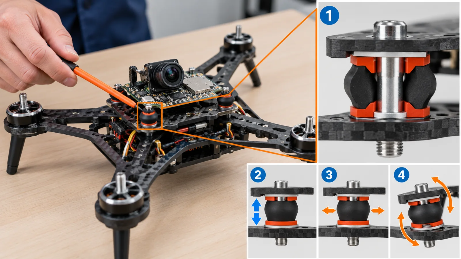
The PX4 documentation explains that flight-controller boards with built-in accelerometers and gyros are sensitive to vibration, and that heavy vibration lowers flight performance, shortens flight time and increases wear, and in extreme cases leads to sensor saturation or failure, estimation failure and loss of control (fly-away) [Reference 13] Sourced. As remedies it lists a frame designed to damp structural resonance, propeller balancing and a vibration-isolating mount for the board (foam and similar), and says it is better to reduce the source of vibration than to remove it with software filters [Reference 13] Sourced. The same advice applies to camera mounting: a VIO camera is very sensitive to vibration, and a soft vibration-isolating mount is recommended [Reference 14] Sourced.

Materials engineer’s view 1: frame material and resonance frequency

As seen in “Fundamentals of Robot Control”, Milenin (2026) measured the resonance peaks of a 7-inch multicopter frame: 147 Hz (no payload) and 204 Hz (2 kg) for cast magnesium AZ31, and 179.5 Hz and 239.4 Hz for aluminium 6061-T6 [Reference 16] Sourced. Frame material and payload move the resonance frequency, and so the vibration frequencies at the place where the IMU sits (commentary). To reduce the vibration spectrum picked up by the IMU and camera, there are materials-side options: use a stiffer material to push resonance to higher frequencies, use a high-damping material, or put a soft material in the mount (commentary). One report found that a magnesium frame had 49% less vibration power than an aluminium frame (2 kg payload, result for a specific design) [Reference 16] Sourced.

2) Materials in front of the sensor, and mounting precision

In front of cameras and LiDAR sit windows, covers and lenses. They need a material that passes the light the sensor uses and resists dirt and scratches (commentary; LiDAR wavelengths and materials are covered in the “LiDAR” article of this series). Also, the relative position and orientation of camera and IMU (extrinsic calibration) is a premise of SLAM. The VINS-Mono paper lists extrinsic calibration among the challenges of monocular VIO, which has no direct distance measurement [Reference 4] Sourced. If the parts holding the sensors move with temperature or shock (thermal expansion, loosening), this calibration may drift and accuracy may fall (inference; we found no quantitative report by material in the sources we checked).

Materials engineer’s view 2: not only “light and stiff” but “does not move, does not shake”

What a sensor mounting plate needs is light weight, stiffness, dimensional stability with temperature, and a property of reducing vibration (commentary). Carbon-fibre composites have high specific stiffness and can be built with low thermal expansion, but as the “Structural Materials for Robots and Drones” article showed, they pass radio waves poorly, so the position of the GNSS antenna needs care. SLAM accuracy rests not only on the performance of the sensor itself but also on the material and structure of its mounting.

9. How to read the yardsticks and standards

SLAM accuracy is measured by how far the trajectory deviates from a ground-truth trajectory. Ground truth comes from motion capture or precise surveying. The main metrics are ATE (absolute trajectory error) and RPE (relative pose error). The TUM RGB-D benchmark explains that ATE suits measuring the performance of a whole SLAM system, and RPE suits measuring the drift of visual odometry (for example per second) [Reference 17] Sourced. Below is what we could confirm (checked 25 October 2026).

Fig. 9 Chart with our calculation (vector drawing). A simulation of a trajectory around a circle of radius 20 m (126 m per lap) where heading error piles up at 1 degree per 10 m. It shows that measuring the same estimate with ATE and RPE gives numbers with different meanings. It is not the result of a real system [Reference 17].

In the example of Fig. 9 the trajectory does not return to its start after one lap, leaving a gap of 4.2 m (about 3.4% of the lap) Our calculation. After global alignment the ATE (RMSE) is 1.26 m, and the RPE over each 10 m segment is 0.085 m (0.84%) Our calculation. It shows that even when local drift is small, it adds up to a large error overall, and that the picture depends on the metric.

Item evaluated	Typical test or benchmark (name, source)	Standards, rules, guidance (ISO, GNSS and so on)	Cautions in reading
Trajectory error (whole SLAM)	TUM RGB-D benchmark: ATE and RPE (Sturm et al., 2012) [17] Sourced	Could not be confirmed	Values change with dataset conditions and the alignment method. ATE is global, RPE is local
Odometry drift	KITTI odometry: ranked by the mean translation error [%] and rotation error [deg/m] over 100 to 800 m segments [18] Sourced. EuRoC MAV dataset (drone data, Burri et al., 2016) [19] Sourced	Could not be confirmed	Rankings are updated. Car-mounted data and small-drone data differ in conditions
Navigation performance of mobile robots	–	ISO 18646-2:2024 “Robotics – Performance criteria and related test methods for service robots – Part 2: Navigation” (2nd edition, January 2024; pose accuracy and repeatability, obstacle detection and avoidance, path deviation, narrow passages, map accuracy; indoor only; not for verifying safety requirements) [20] Sourced. For manipulators, ISO 9283 applies [21] Sourced	Aimed at mobile robots on the ground, not flying robots (a reading of the scope statement; commentary). The text of the standard was not checked
GNSS performance	GPS.gov explanation (smartphone about 4.9 m; FAA data 1.82 m or less [95%]) [10] Sourced	GPS SPS Performance Standard, 5th edition (April 2020; the current edition) [11] Sourced	The commitment is signal quality (URE 2.0 m or less, 95%), not user accuracy
RTK accuracy	DJI Matrice 350 RTK specification: horizontal 1 cm + 1 ppm, vertical 1.5 cm + 1 ppm (RTK FIX) [12] Sourced	Could not be confirmed	Company’s stated values. Changes with baseline length and environment
Vibration and mounting	PX4 documentation (vibration-isolating mount, vibration analysis) [13, 14] Sourced	Could not be confirmed	Vehicle-specific design. No common test method could be confirmed

Standard numbers, titles and status were checked on the official ISO pages (checked 25 October 2026). Standard texts are paid, so we state only the scope. The arrangement of the table is Our calculation. ASTM standard numbers are not covered here because the ASTM site carries a notice prohibiting AI use.

Cautions in reading (for materials engineers)

A dataset accuracy is not accuracy on a real vehicle: “mean 3.6 cm” is a value on indoor EuRoC data. With outdoor conditions, wind, vibration or different light, the number will differ
Check what the quantity means: absolute position error (GNSS), mean trajectory error (ATE), local drift (RPE) and ratio to distance (KITTI) are different quantities
A company’s stated value is not third-party verification: RTK accuracy is a manufacturer’s value under stated conditions
Experimental features are not settled: the PX4 dead-reckoning mode is stated to be experimental as of the check date Not yet confirmed

10. Limits, what could not be confirmed, and summary

What could not be confirmed

Quantitative reports on calibration drift by mounting material: not found. The statement in the text is an inference
Content of LOAM: only the title and bibliography were checked; the text and abstract were not
A common standard for evaluating SLAM: ATE, RPE and KITTI are benchmarks of the research community, not standards. We found no ISO or IEC standard that targets SLAM directly
A standard for evaluating SLAM on drones: ISO 18646-2 reads as aimed at mobile robots on the ground, not flying robots (commentary). No common test method for drones could be confirmed
Text of the GPS SPS Performance Standard: we only confirmed the GPS.gov page description and the edition, and did not read the PDF
ASTM standards: not opened, because the ASTM International site carries a notice prohibiting AI use

Summary

SLAM estimates your position while building a map, and consists of a front end (small motions) and a back end (global optimization) (Fig. 2)
Tracking position with an IMU alone makes error grow with the square of time. An error of 0.01 m/s2 gives 18 m after 60 s Our calculation
Error piles up in proportion to distance travelled (example: 0.61% gives about 6.1 m per km). Returning to the same place (loop closure) lets the whole path be corrected Our calculation
GNSS gives absolute position but is weak indoors and under bridges. SLAM and GNSS complement each other
Drones mostly use camera + IMU (VIO), ground robots a 2D LiDAR. On a drone, sensor mass shortens flight time (+0.5 kg: about 11% less) Our calculation
Frame resonance and mounting materials decide the quality of IMU and camera data. Mounting needs vibration isolation

11. Glossary

SLAM: Simultaneous Localization and Mapping. Estimating own position and building a map at the same time.

Localization: A robot working out its own position and heading within a map.

Six degrees of freedom: Six quantities: three of position (x, y, height) and three of attitude (roll, pitch, yaw).

Odometry: Estimating position by adding up small motions.

Drift: Odometry error piling up over time or distance.

IMU: Inertial measurement unit. Measures motion with accelerometers and gyros (rotation-rate sensors).

GNSS: General name for satellite positioning (GPS and others).

RTK: A method that uses information from a base station to bring GNSS accuracy to a few centimetres.

ppm: Parts per million. “1 cm + 1 ppm” means 1 mm is added per 1 km of baseline.

VIO: Visual-Inertial Odometry. Estimating motion from a camera and an IMU.

LiDAR: A sensor that measures distance with a laser.

Front end: The part of SLAM that estimates small motions from sensor data.

Back end: The part of SLAM that optimizes the path and map together.

Pose graph: A graph with poses as points and relations between motions as lines.

Loop closure: Noticing a return to a place visited before and correcting the whole path’s error.

Occupancy grid: A map divided into cells, each holding whether it is free or occupied.

ATE: Absolute trajectory error. Deviation of the whole estimated trajectory from the true one.

RPE: Relative pose error. Deviation of motion over intervals (the size of drift).

Extrinsic calibration: Finding the relative position and orientation between sensors.

URE: User Range Error. The ranging error carried by the satellite signal.

12. References (primary sources)

Cadena C. et al. “Past, Present, and Future of Simultaneous Localization and Mapping: Toward the Robust-Perception Age”, IEEE Transactions on Robotics 32(6), 1309-1332 (2016), DOI 10.1109/TRO.2016.2624754 (arXiv:1606.05830; checked to the extent of the abstract) – https://arxiv.org/abs/1606.05830
Campos C. et al. “ORB-SLAM3: An Accurate Open-Source Library for Visual, Visual-Inertial, and Multimap SLAM”, IEEE Transactions on Robotics 37(6), 1874-1890 (2021), DOI 10.1109/TRO.2021.3075644 (arXiv:2007.11898; checked to the extent of the abstract) – https://arxiv.org/abs/2007.11898
Scaramuzza D., Zhang Z. “Visual-Inertial Odometry of Aerial Robots”, Encyclopedia of Robotics (2020) (arXiv:1906.03289; checked to the extent of the abstract) – https://arxiv.org/abs/1906.03289
Qin T., Li P., Shen S. “VINS-Mono: A Robust and Versatile Monocular Visual-Inertial State Estimator”, IEEE Transactions on Robotics 34(4), 1004-1020 (2018), DOI 10.1109/TRO.2018.2853729 (arXiv:1708.03852; checked to the extent of the abstract) – https://arxiv.org/abs/1708.03852
Shan T. et al. “LIO-SAM: Tightly-coupled Lidar Inertial Odometry via Smoothing and Mapping”, IEEE/RSJ IROS 2020, 5135-5142, DOI 10.1109/IROS45743.2020.9341176 (arXiv:2007.00258; checked to the extent of the abstract) – https://arxiv.org/abs/2007.00258
Xu W. et al. “FAST-LIO2: Fast Direct LiDAR-Inertial Odometry”, IEEE Transactions on Robotics 38(4), 2053-2073 (2022), DOI 10.1109/TRO.2022.3141876 (arXiv:2107.06829; checked to the extent of the abstract) – https://arxiv.org/abs/2107.06829
Zhang J., Singh S. “LOAM: Lidar Odometry and Mapping in Real-time”, Robotics: Science and Systems X (2014), DOI 10.15607/RSS.2014.X.007 (title and bibliography checked) – https://doi.org/10.15607/RSS.2014.X.007
Hess W., Kohler D., Rapp H., Andor D. “Real-Time Loop Closure in 2D LIDAR SLAM”, IEEE ICRA 2016, 1271-1278, DOI 10.1109/ICRA.2016.7487258 (checked to the extent of the abstract) – https://research.google/pubs/pub45466
Woodman O. J. “An introduction to inertial navigation”, University of Cambridge Computer Laboratory, Technical Report UCAM-CL-TR-696 (2007) (full text checked) – https://www.cl.cam.ac.uk/techreports/UCAM-CL-TR-696.pdf
GPS.gov “GPS Accuracy” (archived version; checked 25 October 2026) – https://archive.gps.gov/systems/gps/performance/accuracy/
GPS.gov “Performance Standards & Specifications” (GPS SPS Performance Standard, 5th edition, April 2020, stated as current; archived version; checked 25 October 2026) – https://archive.gps.gov/technical/ps/
DJI Enterprise “Matrice 350 RTK – Specs” (RTK positioning accuracy; checked 25 October 2026) – https://enterprise.dji.com/matrice-350-rtk/specs
PX4 Autopilot “Vibration Isolation” (PX4 documentation; checked 25 October 2026) – https://docs.px4.io/main/en/assembly/vibration_isolation.html
PX4 Autopilot “Visual Inertial Odometry (VIO)” (PX4 documentation; checked 25 October 2026) – https://docs.px4.io/main/en/computer_vision/visual_inertial_odometry.html
PX4 Autopilot “GNSS-Degraded & Denied Flight (Dead-Reckoning Mode)” (PX4 documentation, v1.17, experimental; checked 25 October 2026) – https://docs.px4.io/main/en/advanced_config/gnss_degraded_or_denied_flight.html
Milenin A. “Experimental Analysis of an AZ31 Magnesium Alloy Structural FPV Drone Frame: Comparison with Aluminum and Carbon Fiber”, Processes 14, 1361 (2026), DOI 10.3390/pr14091361 (open access; checked to the extent of the abstract) – https://doi.org/10.3390/pr14091361
Sturm J. et al. “A benchmark for the evaluation of RGB-D SLAM systems”, IEEE/RSJ IROS 2012, 573-580, DOI 10.1109/IROS.2012.6385773 (ATE and RPE descriptions checked on the evaluation-tools page) – https://cvg.cit.tum.de/data/datasets/rgbd-dataset/tools
Geiger A., Lenz P., Urtasun R. “Are we ready for Autonomous Driving? The KITTI Vision Benchmark Suite”, IEEE CVPR 2012, 3354-3361. Odometry evaluation page (method and ranking; checked 25 October 2026) – https://cvlibs.net/datasets/kitti/eval_odometry.php
Burri M. et al. “The EuRoC micro aerial vehicle datasets”, International Journal of Robotics Research 35(10), 1157-1163 (2016), DOI 10.1177/0278364915620033 (title and bibliography checked) – https://doi.org/10.1177/0278364915620033
ISO “ISO 18646-2:2024 Robotics – Performance criteria and related test methods for service robots – Part 2: Navigation” (ISO standard page) – https://www.iso.org/standard/82643.html
ISO “ISO 9283:1998 Manipulating industrial robots – Performance criteria and related test methods” (ISO standard page) – https://www.iso.org/standard/22244.html
Bauersfeld L., Scaramuzza D. “Range, Endurance, and Optimal Speed Estimates for Multicopters”, IEEE Robotics and Automation Letters (2022, arXiv:2109.04741; hover-power formula checked) – https://arxiv.org/abs/2109.04741

13. Claim-to-source audit

Claim in the text	Basis	Category
Definition of SLAM (building a model of the environment and estimating the robot state at the same time); the survey; the robust-perception age; the standard formulation	Cadena C. et al. Reference 1 https://arxiv.org/abs/1606.05830	Sourced
ORB-SLAM3: visual, visual-inertial and multi-map; mean 3.6 cm on EuRoC with stereo-inertial and 9 mm on handheld TUM-VI; starts a new map when the map is lost and merges it at a known place	Campos C. et al. Reference 1 https://arxiv.org/abs/2007.11898	Sourced
VIO is the only viable way to achieve accurate state estimation without GPS or LiDAR odometry; cameras and IMUs are cheap and on aerial robots	Scaramuzza D., Zhang Z. Reference 1 https://arxiv.org/abs/1906.03289	Sourced
VINS-Mono: monocular camera + IMU is the minimum for metric 6-DOF estimation; no direct distance measurement, so initialization, extrinsic calibration and optimization are challenges; loop detection and 4-DOF pose-graph optimization; closed-loop flight on a vehicle	Qin T., Li P., Shen S. Reference 1 https://arxiv.org/abs/1708.03852	Sourced
LIO-SAM: tightly coupled LiDAR-inertial on a factor graph; IMU integration corrects point-cloud distortion; loop closure and other measurements added as constraints	Shan T. et al. Reference 1 https://arxiv.org/abs/2007.00258	Sourced
FAST-LIO2: iterated Kalman filter; direct registration of points with no feature extraction; ikd-Tree; higher accuracy and lower computation on 19 sequences	Xu W. et al. Reference 1 https://arxiv.org/abs/2107.06829	Sourced
Title and bibliography of LOAM	Zhang J., Singh S. Reference 1 https://doi.org/10.15607/RSS.2014.X.007	Sourced
Cartographer: backpack device; real-time mapping at 5 cm resolution with loop closure; branch-and-bound	Hess W., Kohler D., Rapp H., Andor D. Reference 1 https://research.google/pubs/pub45466	Sourced
Double integration of an acceleration bias e gives position error e t^2 / 2; gyro-noise attitude error is the main cause; over 150 m mean in 60 s with an Xsens MTx IMU (2007)	Woodman O. J. Reference 1 https://www.cl.cam.ac.uk/techreports/UCAM-CL-TR-696.pdf	Sourced
0.01 m/s2 x 3600 / 2 = 18 m; 9.81 x sin 0.1 deg = 0.0171 m/s2; about 31 m	Our calculation (inputs are published values from the sources, or assumptions stated in the text) Reference 1 https://www.cl.cam.ac.uk/techreports/UCAM-CL-TR-696.pdf	Our calculation
Smartphone GPS about 4.9 m under open sky, worse near buildings, bridges and trees; high-quality single-frequency receiver 1.82 m or less at 95% (FAA data); dual-frequency and augmentation give a few cm; the government commitment is signal ranging error (URE) 2.0 m or less (95%), not user accuracy	GPS.gov Reference 1 https://archive.gps.gov/systems/gps/performance/accuracy/	Sourced
GPS SPS Performance Standard, 5th edition (April 2020), is current	GPS.gov Reference 1 https://archive.gps.gov/technical/ps/	Sourced
DJI Matrice 350 RTK: RTK FIX horizontal 1 cm + 1 ppm, vertical 1.5 cm + 1 ppm; mass about 6.47 kg including batteries	DJI Enterprise Reference 1 https://enterprise.dji.com/matrice-350-rtk/specs	Sourced
1 ppm x 10 km = 1 cm, about 2 cm in total (10 km baseline is an assumption)	Our calculation (inputs are published values from the sources, or assumptions stated in the text) Reference 1 https://enterprise.dji.com/matrice-350-rtk/specs	Our calculation
PX4: harm of vibration and sensor saturation; damping of structural resonance; vibration-isolating mount; reduce the source rather than filter	PX4 Autopilot Reference 1 https://docs.px4.io/main/en/assembly/vibration_isolation.html	Sourced
PX4: VIO is used where GPS is missing or uncertain; camera is vibration-sensitive and a soft mount is recommended	PX4 Autopilot Reference 1 https://docs.px4.io/main/en/computer_vision/visual_inertial_odometry.html	Sourced
PX4: dead-reckoning mode (v1.17, experimental, not for flights that start without GNSS, needs another velocity or position sensor)	PX4 Autopilot Reference 1 https://docs.px4.io/main/en/advanced_config/gnss_degraded_or_denied_flight.html	Sourced
Milenin (2026): resonance peaks (AZ31 147 Hz and 204 Hz, aluminium 179.5 Hz and 239.4 Hz); 49% lower vibration power	Milenin A. Reference 1 https://doi.org/10.3390/pr14091361	Sourced
ATE suits whole-SLAM performance and RPE suits visual-odometry drift (TUM RGB-D)	Sturm J. et al. Reference 1 https://cvg.cit.tum.de/data/datasets/rgbd-dataset/tools	Sourced
KITTI: ranked by mean translation error [%] and rotation error [deg/m] over 100 to 800 m segments; one LiDAR method at 0.61%	Geiger A., Lenz P., Urtasun R. Reference 1 https://cvlibs.net/datasets/kitti/eval_odometry.php	Sourced
0.61% means about 6.1 m per 1 km and about 0.61 m per 100 m	Our calculation (inputs are published values from the sources, or assumptions stated in the text) Reference 1 https://cvlibs.net/datasets/kitti/eval_odometry.php	Our calculation
Title and bibliography of the EuRoC MAV datasets	Burri M. et al. Reference 1 https://doi.org/10.1177/0278364915620033	Sourced
ISO 18646-2:2024 (2nd edition, January 2024; pose accuracy and repeatability, obstacles, path deviation, narrow passages, map accuracy; indoor only; not for verifying safety requirements; mobile robots on the ground; manipulators use ISO 9283)	ISO; ISO Reference 1 https://www.iso.org/standard/82643.html Reference 2 https://www.iso.org/standard/22244.html	Sourced
Hover power scales with mass to the power 1.5 (formula)	Bauersfeld L., Scaramuzza D. Reference 1 https://arxiv.org/abs/2109.04741	Sourced
(6.97 / 6.47)^1.5 = 1.118, flight time 1 / 1.118 = 0.894 (0.5 kg is an assumption); 100 m x 100 m at 5 cm is 4.0 x 10^6 cells; 100 x 100 x 10 m at 10 cm is 1.0 x 10^8 cells	Our calculation (inputs are published values from the sources, or assumptions stated in the text) Reference 1 https://research.google/pubs/pub45466 Reference 2 https://arxiv.org/abs/2109.04741	Our calculation
Simulation of Fig. 9: radius 20 m, 1 degree per 10 m, gap 4.2 m (about 3.4%), ATE 1.26 m, RPE 0.085 m (0.84%)	Our calculation (inputs are published values from the sources, or assumptions stated in the text) Reference 1 https://cvg.cit.tum.de/data/datasets/rgbd-dataset/tools	Our calculation
The split into front end and back end; the arrangement of sensor characteristics (general tendencies of LiDAR); how use differs between drone and ground robot (places marked commentary); influence of materials and mounting; calibration drift from thermal expansion or loosening of mounting parts	Commentary (reading not found in a source); our own organization, not the view of any institution	Commentary
How the figures are made: Figs. 2 to 6, 8 and 9 are concept diagrams or charts with our calculation; Figs. 1 and 7 are frames for AI-generated images	Commentary (reading not found in a source); our own organization, not the view of any institution	Commentary
Quantitative reports of calibration drift by material, the content of LOAM, a standard that targets SLAM directly, the text of the GPS SPS standard, ASTM standards	Could not be confirmed in primary sources within the scope of this article, so it is not stated	Commentary

Last updated: 25 October 2026 / Sources are limited to primary sources (peer-reviewed papers and arXiv, a technical report, GPS.gov, PX4 documentation, official benchmark pages, manufacturer specifications, official ISO pages). The curves and numbers in Figs. 4, 5 and 9 come from our own calculation and simulation with stated assumptions, not from values of a specific product or method. The effect of sensor-mounting materials on calibration, the content of LOAM, a standard that targets SLAM directly, and the text of the GPS SPS Performance Standard could not be confirmed, so they are not stated. Figs. 2 to 6, 8 and 9 are concept diagrams or charts with our calculation made for explanation; Figs. 1 and 7 are frames for AI-generated images (no image placed yet).