Closed-Loop Optimization Explained

TECHNOLOGY EXPLAINER

Closed-Loop Optimization
— designing the "propose, experiment, assess, learn" loop to run safely

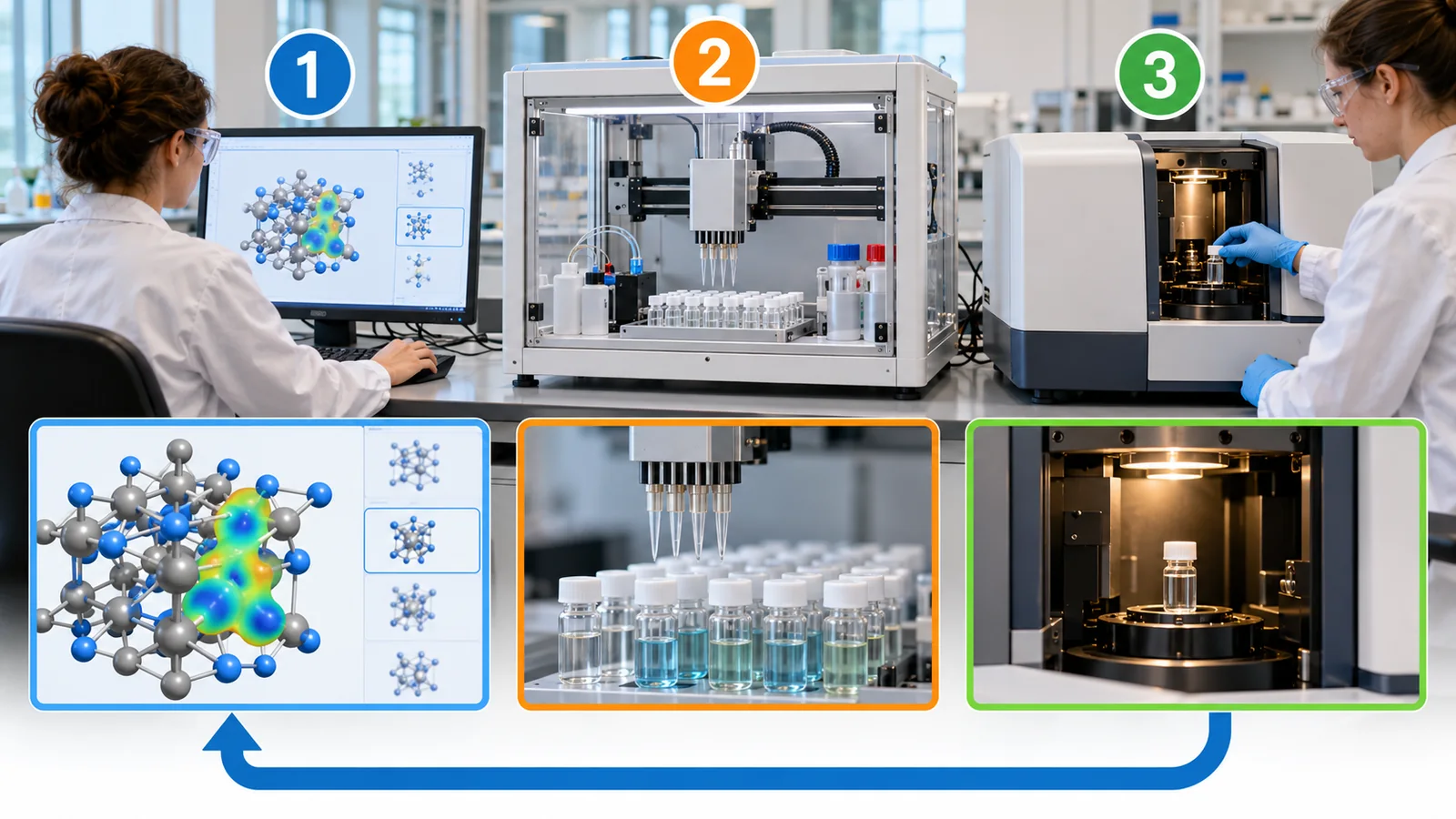
A machine decides the next condition, the experiment is run, the result is learned from and the next condition is decided again. Running this loop moves toward good conditions with few experiments. In reality, though, measurements scatter (noise), some conditions fail and people are still needed. This article explains the inside of the loop (Bayesian optimization) with a small worked example, reads real cases (fast charging of batteries, carbon nanotubes, phase mapping at a synchrotron, toughness of structures, reaction optimization) and sets out four design cautions: measurement noise, constraints and failures, the target metric and human involvement. It is not "add Bayesian optimization and optimization is done" but what it means to design the loop, as far as the papers confirm.

Built from the tutorial by Frazier and papers by Attia et al., Chang et al., Kusne et al., Gongora et al., Shields et al., Rohr et al., Letham et al., Gelbart et al., Häse et al. and Volk and Abolhasani, and official BIPM and ISO pages. Worked numbers are our own calculations. Checked 23 October 2026

Fig. 1. Conceptual illustration generated with ImageGen. 1 choose conditions, 2 prepare the sample, 3 measure it. Feeding results into the next choice distinguishes a closed loop from a fixed automated sequence.Not an actual product, facility or measurement. Enlarged models, lines, arrows and colours are explanatory.

What this article covers

The short version / what to know first / place in the series
Inside the loop: data, model and acquisition function
A small example: how the next point is chosen
Real cases: loops that ran, and speed-up factors
Design caution 1: measurement noise
Design caution 2: constraints and failures
Design caution 3: the target metric and the search range
Design caution 4: human involvement
A design checklist
A materials engineer's view
Limits, what could not be confirmed, and a summary
How to read the yardsticks and standards
Glossary
References
Claim-to-source audit

How claims are labelled in this article

Sourced = stated in published material (link given)
Our calculation = a figure this article derived, with the assumptions spelled out
Not yet confirmed = a plan, target, draft or other item that is not settled
Interpretations for materials engineers are marked separately as commentary; inference is shown in bold; statements by research groups that they "discovered" or "improved" something are labelled as claims.

How to read the numbers in this article

Figures such as "so many times faster" or "a fraction of the experiments" use baselines (exhaustive, grid, random, the authors' own past) that differ from study to study; do not rank methods by the numbers alone. The small example built on an artificial function (Chapter 3) is for showing the mechanism and is not data on any real material.

1. The short version / what to know first / place in the series

Closed-loop optimization is a loop in which a machine chooses the next condition while watching results. Inside it runs data, surrogate model (prediction and uncertainty), acquisition function (value of trying next) and experiment, with Bayesian optimization as the standard exampleSourced[Ref. 1]
Real cases report approaching good conditions with few experiments. For fast charging of batteries, promising conditions among 224 candidates were identified in 16 days (over 500 days by exhaustive search)Sourced[Ref. 3]. But baselines differ from study to study, and noise, failures and human intervention shape the results
The one thing to remember: before running the loop, decide the target metric, the search range and constraints, the noise level and human approval. Taking the maximum of 10 measurements of the same material makes it look about 1.5 sigma above the mean from noise aloneOur calculation

What to know before reading

The ideas of Bayesian optimization and active learning are covered in the series explainer on Bayesian optimization and active learning. Here they are treated as "the part that chooses the next condition", and the article concentrates on design cautions when it is run as a loop. Machine learning is an approximator that learns trends from past data and is weak outside the range of the data (see the explainer on machine-learning basics). The article can be read alone; terms are explained where they first appear.

Place in the series

The machinery by which machines run experiments is in the explainer on self-driving laboratories, making many samples in parallel is in the one on high-throughput experiments and robotic synthesis, and LLMs linking the loop is in the one on AI agents for materials research. This article covers the design of the "decide the next step" loop at their centre. Judging results is in the explainer on evaluation and reproducibility.

2. Inside the loop: data, model and acquisition function

How is "what to try next" decided inside the loop? In Bayesian optimization three things work together.

Fig. 2. Conceptual illustration generated with ImageGen. 1 choose, 2 prepare, 3 measure, 4 record and update. Failed runs also return to the record.Not an actual product, facility or measurement. Enlarged models, lines, arrows and colours are explanatory.

View original SVG, values and sources

Original SVG reference: Conceptual diagram (vector drawing).Frazier (2018) describes Bayesian optimization as building a surrogate of the objective, quantifying its uncertainty and using an acquisition function to decide where to sample next.

Surrogate model: from the conditions and results so far it predicts the result at untried conditions and also counts how uncertain that prediction is. Frazier describes the method using Gaussian process regressionSourced[Ref. 1]
Acquisition function: it scores the value of trying a condition next; a standard one is expected improvement. It balances high predictions (exploitation) against high uncertainty (exploration)Sourced[Ref. 1, 3]
Suitable problems: Frazier says Bayesian optimization suits problems whose evaluation takes a long time, with continuous variables of fewer than 20 dimensions, and tolerates noise in the evaluationSourced[Ref. 1]. Problems outside that (many variables, many categorical variables) need other devices, such as Gryffin, which gives expert knowledge to categorical variablesSourced[Ref. 15]

Easily confused: "exploration" and "exploitation"

Think of choosing a place for lunch. Exploitation is going again to the regular place that has been best so far; exploration is trying a place you have never been to. Only exploiting misses a better place, and only exploring never gets you to a good one. The acquisition function settles this balance with a score. Where the analogy breaks: a meal is judged in one visit, but a materials experiment carries noise, and you must tell whether one "bad" result is truly bad or chance (Chapter 5).

3. A small example: how the next point is chosen

The mechanism is shown with an artificial example in which just one condition is varied. After four experiments the model answers "well known" near the tried points and "not known" far from them. The acquisition function uses that difference to choose the next point.

Fig. 3 Figure including our calculation (vector drawing).The model's prediction after four experiments and how the next point is chosen. In a real self-driving lab there are several variables and the results carry noise.

In the figure the position of the red line was chosen as the next point: a place away from tried points with a high prediction and a large uncertaintyOur calculation. Once the experiment is run, that point adds data, the band narrows and the next point is chosen again. Repeating this is running the loop.

Easily confused: how this example differs from real materials

This example is the simplest case, with one variable, almost no noise and no failures. In reality (1) there are several variables, (2) measurements carry noise, (3) some conditions fail and (4) people restock and approve. The following chapters deal with points 2 to 4.

4. Real cases: loops that ran, and speed-up factors

Case	Target and goal	Experiments and duration	Definition of success and result	Human involvement and verification (as checked)
Attia (2020)	Conditions for six-step, ten-minute fast charging of batteries; maximizing cycle life	Narrowed among 224 candidates in 16 days (over 500 days by exhaustive search without early prediction)Sourced[Ref. 3]	A combination of early prediction (cycle life from the first few cycles) and Bayesian optimizationSourced	The chosen conditions were validated separately (n = 5 each)Sourced[Ref. 3]; the main text is behind a subscription, so human work details were not checked
Chang et al. (2020)	Maximizing the growth rate of carbon nanotubes	About 100 experiments in about 8 hours (5 times faster than the authors' earlier report)Sourced[Ref. 6]	Growth rate up to 8 times that of the seed experimentsSourced	Only the abstract was checked
CAMEO (Kusne et al. 2020)	Phase mapping and property optimization at a synchrotron beamline	Each cycle takes seconds to minutesSourced[Ref. 5]	The authors claim the discovery of a novel epitaxial nanocomposite phase-change memory materialNot yet confirmed	A mode in which a person contributes in each cycle was shownSourced; independent verification was not confirmed
BEAR (Gongora et al. 2020)	Search for the toughness of 3D-printed structures	Almost a 60-fold reduction in the number of experiments relative to a grid-based searchSourced[Ref. 7]	Identified high-performing structures	Only the abstract was checked
Shields et al. (2021)	Optimizing yields of reactions such as a palladium-catalysed one	Compared with an online game of expertsSourced[Ref. 4]	Bayesian optimization outperformed human decision-making in efficiency (number of experiments) and consistency (variance of outcome)Sourced	The aim was a comparison with human decisions; it was also applied to two real reaction optimizationsSourced

Other loops that ran include the mobile robot of Burger et al. (688 experiments in 8 days, batched Bayesian search)Sourced[Ref. 8], Ada (Bayesian optimization by Phoenics, two campaigns of 35 samples)Sourced[Ref. 9] and Coscientist (compared with standard Bayesian optimization)Sourced[Ref. 10] (see the explainers on self-driving laboratories and on AI agents for materials research).

Fig. 4 Figure including our calculation (vector drawing).The speed-up factor changes greatly with the baseline. It must be measured again on your own problem against your own baseline.

The 500 / 16 ≈ 31 of Attia et al. is a lower bound ("over 500 days") against an exhaustive search without early predictionOur calculationSourced[Ref. 3]. It combines another device, early prediction, with the effect of Bayesian optimization
Rohr et al. report, on four chemical spaces of 2,121 catalysts each, an acceleration of up to a factor of 20 against random selection in some scenarios, but also that some choices of model slow the search below randomSourced[Ref. 11]
The Coscientist paper says GPT-4-based approaches scored higher than standard Bayesian optimization, while also noting that the exploration-exploitation balance differs, so this may not indicate performance by itselfSourced[Ref. 10]

Common misconception: "with Bayesian optimization you always reach the optimum in few experiments"

This is not correct. Rohr et al. report that, depending on the choice of model, the search can be slower than random selectionSourced[Ref. 11]. Bayesian optimization also suits some numbers and kinds of variables (continuous or categorical) better than othersSourced[Ref. 1]. The accurate statement is: "with settings that fit the problem it can be faster; compare with random or conventional methods on your own problem."

5. Design caution 1: measurement noise

Measuring the same condition twice gives slightly different values. If this measurement scatter (noise) is ignored, the optimizer chases "lucky measurements". Attia et al. say a battery lifetime experiment can take months to years and that sampling variability is also largeSourced[Ref. 3]. Letham et al. say existing Bayesian optimization degrades when noise is high and propose a method for noisy observations and constraintsSourced[Ref. 12].

Fig. 5 Figure including our calculation (vector drawing).With noise an optimizer can chase "lucky measurements". Attia et al. repeat promising conditions and estimate the uncertainty of results.

In words: even if the materials are all the same (the true difference is 0), taking the maximum of 10 measurements looks about 1.54 sigma (sigma = scatter) above the mean, and for 100 about 2.51 sigmaOur calculation. What is chosen as the "best condition" may be one that happened to measure high. The remedy is to repeat measurements of promising conditions. The method of Attia et al. takes the uncertainty of results (the standard deviation estimated by a Gaussian process) into account in choosing conditions, and it is noted that the protocols with the longest cycle lives have the smallest standard deviations because they were tested repeatedlySourced[Ref. 3].

Easily confused: "noise", "scatter" and "uncertainty"

They are used interchangeably in daily speech, but it helps to separate them. Scatter (noise) is the spread of values when one condition is repeated. Uncertainty is a width expressing how far a value can be trusted. There is an international guide on the idea of measurement uncertainty (the GUM)Sourced[Ref. 21]. ISO 5725-1 is a standard that separates trueness (closeness to the true value) from precision (agreement of repeats)Sourced[Ref. 22] (the text is paid; only the title and scope were checked).

Common misconception: "the condition that measured best is truly the best"

Not necessarily. With noise, the largest measured value tends to be high by an amount of noise (the calculation in the figure). The right check is to repeat the chosen condition on other samples, other days and other lots and see whether the difference exceeds the scatter (sigma) (commentary).

6. Design caution 2: constraints and failures

Optimization is run within the conditions that may be used. Conditions not allowed (safety, equipment limits) can be set by people beforehand. Others, however, are "known to fail only by trying". Gelbart et al. say real problems have constraints unknown beforehand and that noise can enter the evaluation of those constraints tooSourced[Ref. 13].

Fig. 6 Figure including our calculation (vector drawing).If failures are thrown away as "no result" the same region is tried again and again. Failures must be recorded as data ("this condition failed") and reflected in the search (commentary).

Failures really happen: the A-Lab's exception rate averaged about 3.9% across stations over 1.5 yearsSourced[Ref. 19]. In Ada one sample failed in each of the 35-sample campaigns (1 / 35 = about 2.9%)SourcedOur calculation[Ref. 9].
Do not discard failures as "no result": if a failed condition is not recorded the algorithm proposes the same region again. Methods that reflect "this condition failed" in the search (treating it as a constraint) have been studiedSourced[Ref. 13] (commentary).
Limits on the equipment side too: restrict the amounts, temperatures and substances that can be operated outside the algorithm (in equipment or software settings). For safety when the loop affects the physical world, see the "gates" in the explainer on AI agents for materials research

7. Design caution 3: the target metric and the search range

The target metric tends to become a "quickly measurable surrogate": Ada built a "pseudomobility", proportional to hole mobility, from conductance and absorptance of thin films and maximized itSourced[Ref. 9]. Attia et al. used early prediction of lifetime from the first few cycles to shorten each experiment and validated the finally chosen conditions separatelySourced[Ref. 3]. After optimizing on a surrogate, re-check in the final evaluation (commentary)
The search range is set by people: Bayesian optimization chooses the next point within the range given; a good condition outside it will never be visited (commentary). Frazier describes suitable problems as having fewer than 20 continuous dimensionsSourced[Ref. 1]
Bring in expert knowledge: Gryffin gives expert knowledge to categorical variables (catalysts, solvents and so on) in the form of physicochemical descriptors to speed up the search, and is shown on the search for non-fullerene acceptors for organic solar cells, hybrid perovskites and ligandsSourced[Ref. 15]
Tools: implementations of Bayesian optimization include Phoenics (for chemistry)Sourced[Ref. 14] and BoTorch (general)Sourced[Ref. 17]. Olympus is a framework for comparing experiment-planning strategies on data emulating experimentsSourced[Ref. 16].

8. Design caution 4: human involvement

Fig. 7 Conceptual diagram (vector drawing).Based on Kusne et al. (CAMEO, 2020), Shields et al. (2021), Häse et al. (Gryffin, 2021), Dai et al. (2024) and Attia et al. (2020).

People are both outside and inside the loop: CAMEO showed a mode in which a person is called in to contribute within each cycle (human-in-the-loop)Sourced[Ref. 5]. In the mobile-robot run of Dai et al. the only human intervention was restocking and fresh consumablesSourced[Ref. 20].
Human judgment and the algorithm: Shields et al. report that Bayesian optimization outperformed expert chemists and engineers both in the number of experiments and in the scatter of outcomesSourced[Ref. 4]. That compares how experiments are chosen; people still decide the goal, range, constraints, safety and interpretation (commentary).
Processing errors happen too: the Extended Data of Attia et al. candidly note that one protocol that should have been selected in a round was not, owing to a processing errorSourced[Ref. 3]. That is a reason to keep records of the running of the loop (what was chosen and what was executed).

9. A design checklist

The above is condensed into a list of what to decide before running the loop.

Fig. 8 Conceptual diagram (vector drawing).The items are arranged by this article from the statements of Attia et al., Ada, Gelbart et al., Letham et al. and Volk and Abolhasani (commentary).

10. A materials engineer's view

A materials engineer's view 1: measure your own noise (sigma) first

Before running the loop, measure the scatter of your own evaluation by repeating one condition (including lot-to-lot and operator or equipment differences). Once sigma is known you can judge whether an improvement exceeds the scatter. As the calculation in Chapter 5 shows, an improvement within a few sigma can be explained by noise aloneOur calculation. The idea of measurement uncertainty (the GUM) and the distinction between trueness and precision (ISO 5725) help organize this[Ref. 21, 22] (commentary).

A materials engineer's view 2: your past experiments are the best initial data

Bayesian optimization can narrow its aim from the start the more initial data it has. Your lab notebooks, defect reports and past condition tables are valuable initial data that include conditions, results and failures. They are unusable, however, if formats and units are not aligned, so organizing them into numbers, as in the explainer on materials data and descriptors, comes first (commentary). Chang et al. report that good performance was achieved consistently regardless of the number or origin of seed experimentsSourced[Ref. 6].

Fig. 9. Conceptual illustration generated with ImageGen. A failed or constraint-violating run is stopped for review. Define stopping rules and records before trying to accelerate the loop.Not an actual product, facility or measurement. Enlarged models, lines, arrows and colours are explanatory.

A materials engineer's view 3: when a "best" appears, confirm on another day and another lot

The best condition shown by the algorithm is a candidate. Attia et al. validated the chosen conditions with repeats separate from the optimization (n = 5 each, n = 4 for some)Sourced[Ref. 3]. In your own lab confirm with (1) another day, (2) another lot of raw material, (3) another sample preparation and (4) if possible another measurement method. Measuring a control (a known condition) on the same day removes day-to-day variation (commentary). Adopting the condition for a product without this check adopts the "luck" of the noise.

A materials engineer's view 4: decide the stopping rule and the records first

A loop keeps running if left alone. Decide beforehand the limits on count, time and cost, the stopping rule when improvement stalls and who stops it on a fault. For records, keep the model name and version, the settings, the conditions proposed and those executed, failures, lots and the person in charge, tied to sample numbers (see the processing-error example in Chapter 8). The FAIR principles[Ref. 24] help organize records (see the explainer on materials databases and FAIR).

11. Limits, what could not be confirmed, and a summary

(1) What could not be confirmed

The main texts of Attia et al., Chang et al. and Gongora et al. (some behind subscriptions) were checked only through abstracts and Extended Data legends, and human work details and breakdowns of experiments were not checked.
The CAMEO claim of discovering a new material is the authors' claim, and independent verification could not be confirmed.
The review by Shahriari et al. was checked by title only and its content is not described.
Details of optimization software for self-driving labs such as Atlas could not be confirmed here.
Multi-objective optimization and handling of drifting equipment states are not covered here.
An international standard specific to closed-loop optimization was not found. Measurement uncertainty (the GUM, ISO 5725-1) and laboratory competence (ISO/IEC 17025) are neighbouring guides and standards, and since ISO texts are paid only titles were checked.

Summary

Closed-loop optimization is a loop of data, surrogate model, acquisition function and experiment. The next condition is chosen by balancing exploration (uncertain places) and exploitation (places with high predictions)Sourced
The speed-up factors of real cases use different baselines (exhaustive, grid, random, past work), and some settings are slower than randomSourced
Measurement noise: taking the maximum of 10 measurements of the same material looks about 1.5 sigma high from noise alone; confirm by repeatingOur calculation
Design constraints and failures, the surrogate metric, the search range and human involvement outside the loop. Record failures and reflect them in the search (commentary)
The best condition chosen is a candidate. Adopt it only after confirming on another day, another lot and another method (commentary)

12. How to read the yardsticks and standards

The yardsticks of closed-loop optimization are how quickly it approaches good conditions (the speed-up factor) and how far the result can be trusted (quality of measurement and re-confirmation). The factor changes with the baseline, so the baseline must always be stated. Checked on 23 October 2026.

What is assessed	Representative benchmark or method (name, source)	Standards and guidance (ISO/IEC, BIPM, open standards)	How to read it
Speed of search	The acceleration factor (against random selection); Rohr et al.: up to a factor of 20 and, for some choices, slower than random[Ref. 11]Sourced	Not found (no international standard specific to closed-loop optimization was found)	Always check the baseline (exhaustive, grid, random, past work); time and number of experiments are different quantities
Comparison under noisy experiments	Olympus: a framework comparing optimization under noise on probabilistic models emulating experiments[Ref. 16]Sourced	Not found	Performance on emulated experiments differs from performance on your own experiments and depends on the noise level
Measurement uncertainty and accuracy	Experimental precision = the standard deviation of replicates of one condition (Volk and Abolhasani)[Ref. 18]Sourced	JCGM 100:2008 (the GUM, a guide to expressing measurement uncertainty)[Ref. 21]; ISO 5725-1:2023 (accuracy (trueness and precision) of measurement methods and results, Part 1: general principles and definitions)[Ref. 22]Sourced	The GUM is a guide and ISO 5725-1 a standard; neither is a criterion for optimization methods. The ISO text is paid, so only the title and scope were checked
Reliability as a laboratory	Not found	ISO/IEC 17025:2017 (general requirements for the competence of testing and calibration laboratories)[Ref. 23]Sourced	Not a standard for optimization; a reference for thinking about measurement records and traceability (commentary)
Confirming results	Separate validation of chosen conditions (Attia et al.: n = 5 each) and comparison with humans (Shields et al.)[Ref. 3, 4]Sourced	Not found	Write the "best" found in optimization and the value in separate validation separately
Data	Not found	FAIR Guiding Principles (2016)[Ref. 24]Sourced	Principles without legal force; they presuppose metadata on failures and conditions

The arrangement of the table is Our calculation (organization). Numbers, titles and status checked on the ISO and BIPM pages (23 October 2026). Standard texts are paid, so only titles and scope are described and requirements are not.

Reading notes (for materials engineers)

Read "so many times faster" together with its baseline: exhaustive, grid, random and the authors' own past are different baselines. Measure again on your own problem against your own baseline
Separate the best found in optimization from the value in validation: with noise the maximum comes out high. Confirmation on another day and lot is the boundary between a "candidate" and a "confirmed result"
Separate standards from guides and principles: the GUM is a guide, ISO 5725-1 and ISO/IEC 17025 are standards and FAIR is a set of principles. None guarantees that an optimization found a good condition

13. Glossary

Closed-loop optimization: Optimizing conditions by running a loop in which a machine chooses the next condition while watching results.

Bayesian optimization: An optimization method that chooses the next condition from the prediction and uncertainty of a surrogate model.

Surrogate model: A cheap model that predicts results from conditions in place of experiments.

Gaussian process: A kind of surrogate model that gives both a predicted mean and an uncertainty.

Acquisition function: A function that scores the value of trying a condition next.

Expected improvement: An acquisition function for how much better than the current best one can expect.

Exploration and exploitation: Trying uncertain places (exploration) versus trying places with high predictions (exploitation).

Noise (measurement scatter): The spread of measured values when one condition is repeated.

Sigma (standard deviation): A number expressing the size of scatter.

Uncertainty: A width expressing how far a measured value or prediction can be trusted.

Accuracy (trueness and precision): Closeness to the true value (trueness) and agreement of repeats (precision).

Constraint: A limit on usable conditions, such as safety or equipment limits or failure-prone areas.

Surrogate metric: Using a quickly measurable quantity in place of the one you really want.

Early prediction: Predicting the final result (such as lifetime) from the first few cycles to shorten experiments.

Batch (parallel): Choosing several next conditions at once instead of one.

Categorical variable: A variable with non-continuous choices, such as the kind of catalyst or solvent.

Human-in-the-loop: Operation in which a person adds judgment or contribution within the loop.

Baseline: What "so many times faster" is compared with (exhaustive, random, past methods and so on).

Acceleration factor: How many times faster a search reaches a target than random selection.

GUM: The international guide on expressing measurement uncertainty (JCGM 100).

Drift: Slow change of an instrument's state over time.

FAIR principles: Principles for making data findable, accessible, interoperable and reusable.

14. References

Frazier P. I. "A Tutorial on Bayesian Optimization", arXiv:1807.02811 (2018) — arxiv.org/abs/1807.02811
Shahriari B. et al. "Taking the Human Out of the Loop: A Review of Bayesian Optimization", Proc. IEEE 104, 148–175 (2016), DOI 10.1109/JPROC.2015.2494218 (title only) — doi.org/10.1109/JPROC.2015.2494218
Attia P. M. et al. "Closed-loop optimization of fast-charging protocols for batteries with machine learning", Nature 578, 397–402 (2020), DOI 10.1038/s41586-020-1994-5 (abstract and Extended Data legends checked; the main text is behind a subscription) — doi.org/10.1038/s41586-020-1994-5
Shields B. J. et al. "Bayesian reaction optimization as a tool for chemical synthesis", Nature 590, 89–96 (2021), DOI 10.1038/s41586-021-03213-y — doi.org/10.1038/s41586-021-03213-y
Kusne A. G. et al. "On-the-fly closed-loop materials discovery via Bayesian active learning", Nat. Commun. 11, 5966 (2020), DOI 10.1038/s41467-020-19597-w — doi.org/10.1038/s41467-020-19597-w
Chang J. et al. "Efficient Closed-loop Maximization of Carbon Nanotube Growth Rate using Bayesian Optimization", Sci. Rep. 10, 9040 (2020), DOI 10.1038/s41598-020-64397-3 — doi.org/10.1038/s41598-020-64397-3
Gongora A. E. et al. "A Bayesian experimental autonomous researcher for mechanical design", Sci. Adv. 6, eaaz1708 (2020), DOI 10.1126/sciadv.aaz1708 — doi.org/10.1126/sciadv.aaz1708
Burger B. et al. "A mobile robotic chemist", Nature 583, 237–241 (2020), DOI 10.1038/s41586-020-2442-2 (abstract checked) — doi.org/10.1038/s41586-020-2442-2
MacLeod B. P. et al. "Self-driving laboratory for accelerated discovery of thin-film materials", Sci. Adv. 6, eaaz8867 (2020), DOI 10.1126/sciadv.aaz8867 — doi.org/10.1126/sciadv.aaz8867
Boiko D. A., MacKnight R., Kline B., Gomes G. "Autonomous chemical research with large language models", Nature 624, 570–578 (2023), DOI 10.1038/s41586-023-06792-0 — doi.org/10.1038/s41586-023-06792-0
Rohr B. et al. "Benchmarking the acceleration of materials discovery by sequential learning", Chem. Sci. 11, 2696–2706 (2020), DOI 10.1039/C9SC05999G — doi.org/10.1039/C9SC05999G
Letham B. et al. "Constrained Bayesian Optimization with Noisy Experiments", Bayesian Anal. 14, 495–519 (2019), DOI 10.1214/18-BA1110 (abstract checked in arXiv:1706.07094) — arxiv.org/abs/1706.07094
Gelbart M. A., Snoek J., Adams R. P. "Bayesian Optimization with Unknown Constraints", arXiv:1403.5607 (2014) — arxiv.org/abs/1403.5607
Häse F. et al. "Phoenics: A Bayesian Optimizer for Chemistry", ACS Cent. Sci. 4, 1134–1145 (2018), DOI 10.1021/acscentsci.8b00307 — doi.org/10.1021/acscentsci.8b00307
Häse F. et al. "Gryffin: An algorithm for Bayesian optimization of categorical variables informed by expert knowledge", Appl. Phys. Rev. 8, 031406 (2021), DOI 10.1063/5.0048164 — doi.org/10.1063/5.0048164
Häse F. et al. "Olympus: a benchmarking framework for noisy optimization and experiment planning", Mach. Learn.: Sci. Technol. 2, 035021 (2021), DOI 10.1088/2632-2153/abedc8 — doi.org/10.1088/2632-2153/abedc8
Balandat M. et al. "BoTorch: A Framework for Efficient Monte-Carlo Bayesian Optimization", arXiv:1910.06403 (2019) — arxiv.org/abs/1910.06403
Volk A. A., Abolhasani M. "Performance metrics to unleash the power of self-driving labs in chemistry and materials science", Nat. Commun. 15, 1378 (2024), DOI 10.1038/s41467-024-45569-5 — doi.org/10.1038/s41467-024-45569-5
Szymanski N. J. et al. "An autonomous laboratory for the accelerated synthesis of inorganic materials", Nature 624, 86–91 (2023), DOI 10.1038/s41586-023-06734-w (version reflecting the January 2026 correction) — doi.org/10.1038/s41586-023-06734-w
Dai T. et al. "Autonomous mobile robots for exploratory synthetic chemistry", Nature 635, 890–897 (2024), DOI 10.1038/s41586-024-08173-7 — doi.org/10.1038/s41586-024-08173-7
JCGM "JCGM 100:2008 Evaluation of measurement data — Guide to the expression of uncertainty in measurement (GUM)" (BIPM publications page, checked 23 October 2026; a 2026 Amendment 1 is listed on the same page) — bipm.org/en/committees/jc/jcgm/publications
ISO "ISO 5725-1:2023 Accuracy (trueness and precision) of measurement methods and results — Part 1: General principles and definitions" (ISO page) — iso.org/standard/69418.html
ISO/IEC "ISO/IEC 17025:2017 General requirements for the competence of testing and calibration laboratories" (ISO page) — iso.org/standard/66912.html
Wilkinson M. D. et al. "The FAIR Guiding Principles for scientific data management and stewardship", Sci. Data 3, 160018 (2016), DOI 10.1038/sdata.2016.18 — doi.org/10.1038/sdata.2016.18

15. Claim-to-source audit

Claim in the text	Basis	Class
Frazier: the surrogate (Gaussian process regression) and uncertainty, acquisition functions (expected improvement and others), suited to long-to-evaluate problems with fewer than 20 continuous dimensions, tolerance of noise, extensions to parallel evaluation and constraints. The title of the review by Shahriari et al.	Reference 1 https://arxiv.org/abs/1807.02811 Reference 2 https://doi.org/10.1109/JPROC.2015.2494218	Sourced
Attia et al.: six-step, ten-minute fast charging, narrowing among 224 candidates in 16 days (over 500 days by exhaustive search without early prediction), early prediction, Bayesian optimization, large sampling variability, protocols with the longest lives tested repeatedly with small standard deviations, separate validation of chosen conditions (n = 5 each, n = 4 for some), one protocol not selected owing to a processing error, exclusion of failed batteries	Reference 3 https://doi.org/10.1038/s41586-020-1994-5	Sourced
Chang et al.: carbon nanotube growth rate up to 8 times that of the seed experiments, about 100 experiments in about 8 hours (5 times faster than the earlier report), consistent regardless of the number or origin of seed experiments. Gongora et al. (BEAR): almost a 60-fold reduction in experiments relative to a grid-based search	Reference 6 https://doi.org/10.1038/s41598-020-64397-3 Reference 7 https://doi.org/10.1126/sciadv.aaz1708	Sourced
Kusne et al. (CAMEO): a closed loop at a synchrotron beamline, each cycle taking seconds to minutes, a mode in which a person contributes in each cycle, the authors' claim of discovering a novel epitaxial nanocomposite phase-change memory material	Reference 5 https://doi.org/10.1038/s41467-020-19597-w	Not yet confirmed
Shields et al.: Bayesian optimization outperforming expert chemists and engineers in efficiency (number of experiments) and consistency (variance of outcome), an online game, application to two real reactions	Reference 4 https://doi.org/10.1038/s41586-021-03213-y	Sourced
Rohr et al.: four chemical spaces of 2,121 catalysts each, up to a factor of 20 against random selection, slower than random for some choices. Burger et al.: 688 experiments in 8 days with a batched Bayesian search. Ada: Phoenics, 35 samples, the pseudomobility. Coscientist: comparison with standard Bayesian optimization and its caveat	Reference 11 https://doi.org/10.1039/C9SC05999G Reference 8 https://doi.org/10.1038/s41586-020-2442-2 Reference 9 https://doi.org/10.1126/sciadv.aaz8867 Reference 10 https://doi.org/10.1038/s41586-023-06792-0	Sourced
Letham et al.: existing Bayesian optimization degrades when noise is high, a method for noisy observations and constraints. Gelbart et al.: constraints unknown beforehand, noise possibly entering the evaluation of constraints	Reference 12 https://arxiv.org/abs/1706.07094 Reference 13 https://arxiv.org/abs/1403.5607	Sourced
Phoenics (Bayesian optimization for chemistry), Gryffin (expert knowledge for categorical variables; examples of non-fullerene acceptors, perovskites and ligands), Olympus (a framework for comparing noisy optimization on emulated experiments), BoTorch	Reference 14 https://doi.org/10.1021/acscentsci.8b00307 Reference 15 https://doi.org/10.1063/5.0048164 Reference 16 https://doi.org/10.1088/2632-2153/abedc8 Reference 17 https://arxiv.org/abs/1910.06403	Sourced
Volk and Abolhasani: experimental precision as the standard deviation of replicates. A-Lab: exception rate averaging about 3.9% across stations over 1.5 years. Dai et al.: human intervention limited to restocking and consumables	Reference 18 https://doi.org/10.1038/s41467-024-45569-5 Reference 19 https://doi.org/10.1038/s41586-023-06734-w Reference 20 https://doi.org/10.1038/s41586-024-08173-7	Sourced
The title of JCGM 100:2008 (the GUM) and the listing of a 2026 Amendment 1 on the BIPM page; the number, title and status (published, Edition 2, July 2023) of ISO 5725-1:2023; the title and status of ISO/IEC 17025:2017; the FAIR Guiding Principles (2016)	Reference 21 https://www.bipm.org/en/committees/jc/jcgm/publications Reference 22 https://www.iso.org/standard/69418.html Reference 23 https://www.iso.org/standard/66912.html Reference 24 https://doi.org/10.1038/sdata.2016.18	Sourced
The expected maximum of N standard normal values (0, 0.56, 1.16, 1.54, 1.87, 2.25 and 2.51 sigma for N = 1, 2, 5, 10, 20, 50 and 100), about 7.7% for ten measurements when sigma is 5%; 500 / 16 ≈ 31 and 1 / 35 ≈ 2.9%; the prediction, uncertainty, expected improvement and next point of the small example (f(x) = sin(3x) + 0.5x, RBF kernel length scale 0.45)	Our calculation (Python; numerical integration and Gaussian process computation)	Our calculation
Details in the main texts of Attia et al., Chang et al. and Gongora et al.; independent verification of CAMEO; the content of the review by Shahriari et al.; details of software such as Atlas; multi-objective optimization and drift; an international standard specific to closed-loop optimization	Not confirmed in the primary sources reachable in this survey, so not stated	Commentary
The readings "re-check a surrogate in the final evaluation", "people set the search range", "record failures and reflect them in the search", "measure your own sigma first", "use past experiments as initial data", "confirm the best condition on another day and lot", "decide the stopping rule and records first", the checklist of Fig. 8 and the way speed-up factors are arranged in Fig. 4	Our own arrangement and commentary based on published material; not a view stated by the researchers or institutions	Commentary
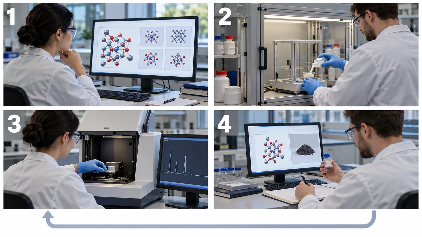
Figs. 2 (loop), 7 (human involvement) and 8 (checklist) are conceptual diagrams; Figs. 3 (worked example), 4 (speed-up), 5 (noise) and 6 (constraints and failures) include calculations (the bars of Fig. 4 are published factors, with only 500 / 16 our calculation); Figs. 1 and 9 are slots for AI-generated images; the small example in Fig. 3 is an artificial function and not data on a real material	Note by this article	Commentary

Last updated: 23 October 2026. Sources are limited to primary material (peer-reviewed papers, arXiv papers, and official BIPM and ISO pages). Worked numbers are our own calculations, not results of actual experiments. Details in the main texts of Attia et al., Chang et al. and Gongora et al., independent verification of CAMEO, details of software such as Atlas, multi-objective optimization and drift, and an international standard specific to closed-loop optimization could not be confirmed and are not stated. Figs. 1 and 9 are slots for AI-generated images; the other figures are explanatory diagrams or figures including calculations.