TECHNOLOGY EXPLAINER
High-Throughput Computation
Running many candidates through automated workflows to narrow them down
"There are tens of thousands of candidate materials. We cannot test them all in the lab." So a method arose that computes candidates one after another by computer and sends only the promising ones to experiment. It is high-throughput computation (HTC), and databases such as the Materials Project are built this way. This article uses figures and simple calculations to explain the machinery for running calculations automatically in large numbers (workflows) and the flow of screening that narrows candidates. It then sets out, from a materials engineer's viewpoint, the cost of the calculations, how "promising" is judged (the convex hull) and how reliable the calculations are. How to read DFT itself is covered in our explainer on the fundamentals of density functional theory, so here we concentrate on what is specific to running calculations in bulk.
- The short version, what to know first, and where this fits in the series
- What high-throughput computation is
- The flow of screening
- Automating one calculation: workflows
- Estimating the computational cost
- How "promising" is judged: the convex hull
- How reliable are the calculations?
- Databases and how they are shared
- Screening examples
- A materials engineer's view
- Limits, what we could not confirm, and a summary
- How to read the yardsticks and standards
- Glossary
- References
- Claim-to-source audit
Sourced = stated in a published source (linked)
Our calculation = a value computed in this article from the stated assumptions
Not yet confirmed = plans, targets, drafts, work in progress, outlooks: not settled
Our own reading for materials engineers is marked as commentary. Inference is shown in bold. Computed predictions and results confirmed by experiment are kept apart.
1. The short version, what to know first, and where this fits in the series
- High-throughput computation runs the calculations for many candidates automatically through workflows, accumulates the results in a database, and narrows down the promising candidates. The Materials Project began as a program to use this approach to compute and publish the properties of known inorganic materials Sourced[Ref. 1]. The project says that, more than a decade after its launch, it is used by more than 600,000 researchers Sourced[Ref. 2]
- The key is "filter cheaply first, and spend the costly calculations only on the remaining candidates". In our example based on assumptions (our calculation), screening 100,000 candidates with a funnel cost about one twenty-fifth of running DFT on all of them Our calculation. But the risk of discarding good candidates by filtering is not included in that figure
- "Stable" by calculation does not mean "can be made", and computed values change with conditions. When the same structures were computed in three databases, formation energies differed by up to 0.105 eV/atom Sourced[Ref. 3]. Calculation produces candidates; experiment confirms whether they are real
In the series' common analogy, materials search is "looking for treasure on a vast map", and the combinations are too many to try all. High-throughput computation is a tool that surveys a wide area of the map automatically by machine and narrows down where the treasure may be. In the division of labour in which calculation produces candidates cheaply and quickly, experiment confirms whether they are real, and AI narrows where to look, this article is mainly about the "calculation" part. DFT is "a physics simulation that computes properties from the behaviour of electrons"; it contains approximations and need not agree with measurement.
A good order is our explainers on the fundamentals of density functional theory (how to read DFT) and on materials databases and the FAIR principles (where computed data are kept), then this article (the machinery for computing in bulk). Using AI to speed up the early narrowing is covered in our explainers on machine-learning interatomic potentials and graph neural networks, and automating the experiments that come after calculation in the explainers on high-throughput experiments and robotic synthesis and on self-driving laboratories.
2. What high-throughput computation is
Picture the inspection line of a factory. Products keep flowing in, machines carry out the same checks automatically, and only those that pass go on to the next step. High-throughput computation is like putting "candidate materials" on an inspection line. For each candidate, the machine automatically repeats the same procedure: fix the structure, compute the energy, compute the properties.
- Origins: the Materials Project began as a core program of the Materials Genome Initiative, using high-throughput computing to uncover the properties of known inorganic materials Sourced[Ref. 1]. It says it was formally launched in 2011 Sourced[Ref. 2].
- A review: the review by Curtarolo et al. introduces the field as one that combines advanced thermodynamic and electronic-structure methods with data mining, database construction and supercomputers to generate enormous data repositories and use them for discovery Sourced[Ref. 4].
- Main computational databases: the Materials Project, AFLOW (Curtarolo et al. 2012), OQMD (nearly 300,000 DFT total-energy calculations, per its 2015 paper), JARVIS-DFT (about 40,000 materials and about 1 million calculated properties, per its 2020 paper) and others Sourced[Refs. 5, 6, 7].
A factory inspection has clear pass-or-fail standards, such as dimensions. But the "inspection" in calculation is DFT, a calculation that contains approximations. Even when the result says "pass" (stable, a suitable gap and so on), it remains a hypothesis until confirmed by experiment. The chapter on reliability covers this in more detail.
3. The flow of screening
The basis of high-throughput computation is "narrow in stages, cheapest first". A single DFT calculation is not cheap (hours to days). So at the start, rules and cheap estimates cut the candidates sharply.
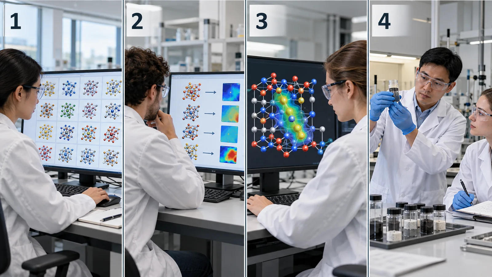
View original SVG, values and sources
Original SVG reference: Concept diagram (vector drawing). The screening flow of high-throughput computing: cheap stages cut the candidates sharply, and costly calculations are spent only on those that remain.
- Generate candidates: prepare compositions and crystal structures in bulk. Methods such as substituting elements in known crystal structures are used.
- Filter by rules: for example, check whether the charges of a compound balance and whether the elements are usable. Davies et al. showed that four-component compounds from the first 103 elements number more than 10¹² combinations, and that removing chemically implausible compositions with the principles of valency and electronegativity reduces the inorganic quaternary space to 10¹⁰ Sourced[Ref. 8].
- Cheap estimates: narrow further with machine learning and similar tools (Matbench Discovery evaluates machine-learning energy models as pre-filters for stable crystals Sourced[Ref. 9]).
- DFT calculation: relax the structure and compute the energy for the remaining candidates.
- Judge stability: look at the energy above the convex hull (a later chapter).
- Target properties: compute band gaps, ease of ion motion, phonons and so on.
- To experiment: synthesise a few candidates and check them.
"Throughput" is the amount that can be processed per unit time. High-throughput computation stresses not "making one calculation faster" but "running a great many calculations automatically without stopping". So the star is not the accuracy of any single calculation but the machinery that runs the calculations automatically and keeps the results in order (commentary).
4. Automating one calculation: workflows
It is impossible for people to submit tens of thousands of calculations one by one. So tools for workflow management are used. One calculation (structure relaxation, then a static calculation, then property calculations) is a chain of several jobs, and it can fail partway.
- FireWorks (Jain et al. 2015): workflow software for high-throughput calculations at supercomputing centres, reported to have been used for over 50 million CPU-hours of calculation at the National Energy Research Scientific Computing Center (NERSC). It supports concurrent execution (job packing), failure detection and correction, provenance (how a result was made) and reporting, automated duplicate detection, and changes to a workflow while it runs Sourced[Ref. 10].
- atomate and pymatgen: atomate is a high-level interface to generate, execute and analyze computational materials science workflows, and pymatgen is a robust open-source Python library for materials analysis (by their titles) Sourced[Refs. 11, 12].
- AiiDA: an open-source high-throughput infrastructure for automated workflow management and recording data provenance. AiiDA 1.0 supports throughputs of tens of thousands of processes per hour and stores the full provenance in a queryable database Sourced[Ref. 13]. Its workflow engine is designed to scale from an individual laptop to supercomputers and to manage jobs with runtimes from fractions of a second to weeks, with thousands of jobs concurrently Sourced[Ref. 14].
When you use values from a database, the most troublesome thing is "not knowing what settings produced that value". If the workflow automatically records the input structure, the functional, U, the pseudopotential and the software version, you can later pick only values under the same conditions and compare them. When you run calculations in-house, set up first a mechanism that keeps the settings and versions together with the results (provenance). It points the same way as the FAIR principles (data that are findable, accessible, interoperable and reusable) Sourced[Ref. 15].
5. Estimating the computational cost
What does "computing in bulk" cost? As a guide to real scale, the FireWorks paper reports over 50 million CPU-hours of calculation. Running 1,000 cores without a break, that is about 5.7 years Our calculation (50 million ÷ (1,000 × 8,760 hours)).
- We calculated with the following example (all assumptions are for explanation). Of 100,000 candidates, rules (0.001 core-hours each) leave 20,000, a cheap estimate (0.1 core-hours) leaves 2,000, DFT (100 core-hours) leaves 200, and detailed properties (1,000 core-hours) leave 20 to go to experiment Our calculation.
- The total is about 402,000 core-hours, about one twenty-fifth of the 10 million core-hours needed to run DFT on all 100,000. On 1,000 cores that is about 17 days against about 417 days Our calculation.
- What this calculation leaves out: the risk of discarding genuinely good candidates by filtering (misses), the cost of failed calculations and reruns, and people's time.
The early narrowing is not a "replacement" for DFT; it reduces how many calculations DFT must do. Bartel et al. report that even when machine learning predicts formation energy well, models using only the composition do poorly at the "stable or not" decision, and that in sparse chemical spaces only a structural model found stable materials efficiently Sourced[Ref. 16]. The authors of Matbench Discovery also point out a misalignment between regression metrics and decision metrics, and say that universal interatomic potentials have advanced enough to serve as pre-filters Sourced[Ref. 9]. The final judgement is made with DFT (and then experiment).
6. How "promising" is judged: the convex hull
The first criterion used in screening is stability. As a first guide to "can it be made?", calculation uses the convex hull.
- The convex hull: for a combination of elements (say A and B), it is the lower line that shows, from formation energies, "which compound is the most stable at which composition". Compounds on the hull are predicted to be thermodynamically stable.
- Energy above hull: how far above the hull a compound lies. The Materials Project glossary explains that this is a 0 K prediction without a temperature axis; that materials on the hull are predicted stable and those off it metastable or unstable; and that values above 200 meV/atom are very large and suggest a material that might not be synthesizable, though this ceiling differs significantly by chemistry Sourced[Ref. 17].
- Metastable compounds can sometimes be made: Sun et al. studied the thermodynamic scale of metastability for 29,902 known crystalline phases in the Materials Project, and argued that not all low-energy metastable compounds can necessarily be synthesized, and that observable metastable phases are generally remnants of conditions where they were once the lowest free-energy phase Sourced[Ref. 18].
A real phase diagram changes with temperature and pressure. The convex hull is a diagram built at 0 K, from DFT total energies alone. It leaves out entropy (important at high temperature), vibrations, defects and surface effects. So even when the energy above the hull is small, the real phase can change with high temperature or synthesis conditions (commentary).
7. How reliable are the calculations?
You can trust the result of narrowing only when the calculation error is smaller than the width of the decision. Let us put published errors on the same ruler (meV/atom).
- DFT against experiment: in the OQMD check, the mean absolute error against 1,670 experimental formation energies was 0.096 eV/atom, and the disagreement among experiments themselves was 0.082 eV/atom Sourced[Ref. 5].
- Between databases: Hegde et al. showed that between AFLOW, the Materials Project and OQMD, formation energies differ by up to 0.105 eV/atom (median about 6%), band gaps by up to 0.21 eV (about 9%), and the verdicts on whether a material is a metal and whether it is magnetic disagree for up to 7% and 15% of records. The size of the differences was comparable to the difference between DFT and experiment, and the causes were the choice of pseudopotentials, DFT+U and the elemental reference states Sourced[Ref. 3].
- Mixing different functionals: the Materials Project mixes PBE (GGA), DFT+U and r²SCAN calculations through energy corrections and places them on one phase diagram Sourced[Ref. 19]. Kingsbury et al. showed how to combine "higher-fidelity, low-coverage calculations" robustly with "lower-fidelity, high-coverage calculations" Sourced[Ref. 20].
- Agreement between codes: Lejaeghere et al. showed that recent codes and pseudopotentials agree very well on 71 elemental crystals Sourced[Ref. 21].
If the calculation error is about 0.1 eV/atom (100 meV/atom), it is risky to call something stable or unstable on a difference of a few tens of meV/atom in the energy above the hull. For candidates "very close to the hull", check: (1) does a different functional (r²SCAN and so on) give the same verdict; (2) do several databases agree; (3) is the phase actually formed in experiment. It is realistic to use the threshold not as a "stable/unstable" line but as a guide to the priority for experimental confirmation (commentary).
8. Databases and how they are shared
Computed results are stored in databases and shared. Here are the main ones, as far as we could confirm.
| Database / infrastructure | Scale and features we could confirm | Reading note |
|---|---|---|
| Materials Project | Formally launched in 2011; used by more than 600,000 researchers (2025 perspective); latest version v2026.09.28 (live on 19 October 2026) Sourced[Refs. 2, 22] | Normally PBE (GGA). Recomputation with r²SCAN is under way. Values change between versions |
| OQMD | Nearly 300,000 DFT total-energy calculations (2015 paper). The data are released without restrictions (as stated in the paper) Sourced[Ref. 5] | Scale as of the paper. We did not check the current count |
| JARVIS-DFT | About 40,000 materials and about 1 million calculated properties (2020 paper). Evaluates errors by comparing computed data with experiments or high-fidelity calculations Sourced[Ref. 6] | Scale as of the paper |
| AFLOW | An automatic framework for high-throughput materials discovery (Curtarolo et al. 2012) Sourced[Ref. 7] | We did not check the current scale |
| GNoME data | About 381,000 crystals on the updated convex hull (computed). 74,052 GNoME-derived materials computed with r²SCAN were added to the Materials Project, for a total of 117 thousand (April 2026 entry) Sourced[Refs. 23, 22] | Computed predictions. Synthesizability is a separate question |
The arrangement of the table is Our calculation (organisation). Check the official pages for the licence and terms of use of each database (we did not check them here, except for statements in some papers). Checked on 23 October 2026.
If every database has its own way of being queried, searching across them is hard. The OPTIMADE consortium designed a universal API to make materials databases interoperable, and reports that its first stable specification, v1.0, is supported by many leading databases and several software packages Sourced[Ref. 24]. But a common door only makes data "easier to find"; it does not remove the differences in calculation settings between databases.
9. Screening examples
We set side by side examples in which calculation narrowed candidates and experiment confirmed them, and examples of computed predictions. All are reports (claims) by the research groups.
| Study | Target and method | What was reported | Reading note |
|---|---|---|---|
| Greeley et al. (2006) | Electrocatalysts for hydrogen evolution. High-throughput DFT screening | The activity of over 700 binary surface alloys was computed, and the stability of each in electrochemical environments was estimated. BiPt was predicted to have activity comparable to or better than Pt; when synthesised and tested it showed improved hydrogen-evolution performance compared with Pt, in agreement with the screening Sourced[Ref. 25] | An example narrowed by calculation and confirmed by experiment. What was confirmed was one alloy from the narrowed set |
| Hautier et al. (2010) | Unknown ternary oxide compounds. A probabilistic model built from an experimental crystal-structure database, plus DFT | The model chose compositions and structures likely to form compounds, DFT tested their stability, and 209 new compounds were found with a limited computational budget Sourced[Ref. 26] | Computed predictions (the paper's word is "discovering"). Not a synthesis result |
| Davies et al. (2016) | All stoichiometric inorganic materials. Rules of valency and electronegativity | Reduced more than 10¹² quaternary combinations to 10¹⁰ and used the approach to search for perovskites and the like. Because the approach is simple, large-scale searches can run on a single workstation Sourced[Ref. 8] | A coarse filter using composition only |
| Merchant et al. (2023) | Active learning with GNNs and DFT (GNoME) | About 2.2 million structures were computed to be stable relative to earlier data, about 381,000 of them on the updated hull, and 736 match existing experimental reports Sourced[Ref. 23] | Computed predictions and matches with existing experimental reports. See our graph neural network explainer for details |
Each number is a value under the conditions of its own paper. The arrangement of the table is Our calculation (organisation). Checked on 23 October 2026.
10. A materials engineer's view
What to feed into high-throughput computation is for the engineer to decide. Organise it in this order: (1) turn the pass conditions into numbers (for example, energy above hull of 50 meV/atom or less, a gap of 1.5 to 2.5 eV, no toxic elements); (2) put the non-negotiable constraints in first (resources, cost, toxicity, availability); (3) set priorities among properties (weights for several properties); (4) leave conditions unsuited to calculation (performance that depends on microstructure or process) to the experimental side. Set the calculated "pass" line looser, with the calculation error (about 0.1 eV/atom) in mind, to reduce missed candidates (commentary).
If you test only the candidates at the top of the calculation, you cannot tell whether the calculation was right. In addition to (1) the top candidates, synthesise and measure (2) candidates ranked low by calculation, and known materials (controls) under the same conditions. Then check in turn (3) was the target phase obtained (telling it from known compounds or solid solutions, for example by powder X-ray diffraction), (4) does it reproduce (another lot), and (5) the effect of impurities and disorder. Keeping the results as a table of "calculated prediction against measurement" gives material for setting the thresholds of the next screening (commentary).
11. Limits, what we could not confirm, and a summary
(1) What we could not confirm
- We did not confirm the current scale and the licences of OQMD, AFLOW and JARVIS-DFT (scale is as of the papers).
- We did not confirm what happened afterwards in synthesis to the 209 compounds of Hautier et al.
- We did not confirm experimental confirmation of the candidates actually found in the narrowing of Davies et al.
- Our cost estimate is an example based on assumptions; it does not include the cost of real studies or the miss rate.
- We could not confirm an international standard (ISO/IEC or similar) specific to high-throughput computation.
- High-throughput computation runs calculations automatically in bulk through workflows, keeps the results in databases, and narrows down promising candidates. Workflow tools handle failure detection and resubmission, and the recording of provenance Sourced
- The key is to narrow cheapest-first. In our example the cost was about one twenty-fifth of running DFT on every candidate. The risk of misses is not included Our calculation
- Stability is judged by the energy above the convex hull. It is a 0 K prediction; metastable compounds can sometimes be made, and stable ones cannot always be Sourced
- The calculation error (about 0.1 eV/atom) can be close to the width of the decision. Even databases disagree on gaps and magnetism Sourced
- Calculation produces candidates and experiment confirms them. Measure controls as well as the top candidates, and keep the correspondence between calculation and measurement Sourced
12. How to read the yardsticks and standards
The first yardstick of high-throughput computation is the performance of the narrowing (the hit rate: the share of predicted candidates that were actually stable). Next come the reliability of the calculations (errors, agreement between databases) and reproducibility and sharing (are the settings and provenance kept, can the data be found). Even a high hit rate is a hit rate for "computed stability", not an experimental success rate. Checked on 23 October 2026.
| Item | Representative benchmarks and methods (name, source) | Standards and guidance (ISO/IEC, NIST, etc.) | Reading notes |
|---|---|---|---|
| Performance of narrowing (hit rate) | GNoME: over six rounds of active learning, the share of correct stable predictions rose from under 6% to over 80% for structural models and from under 3% to 33% for compositional models (Merchant et al.) [Ref. 23]Sourced Matbench Discovery: evaluates machine-learning energy models as pre-filters (Riebesell et al. 2025) [Ref. 9]Sourced | Not found (we did not find an international standard defining how to evaluate high-throughput screening) | "Stable" is a DFT (PBE), 0 K verdict. It is not an experimental success rate |
| Judging stability | Energy above the convex hull (Materials Project glossary) [Ref. 17]Sourced. The accuracy of formation energies and the accuracy of stability decisions differ (Bartel et al. 2020) [Ref. 16]Sourced | Not found | Thresholds differ by chemistry. Allow for the error (about 0.1 eV/atom) |
| Reliability of calculations | Comparison between databases (Hegde et al. 2023) [Ref. 3]. Comparison of OQMD with experiment (Kirklin et al.) [Ref. 5]. Agreement between codes (Lejaeghere et al. 2016) [Ref. 21] Sourced | Not found | Gaps and magnetism tend to disagree |
| Reproducibility and sharing | The FAIR principles (Wilkinson et al. 2016) [Ref. 15]. Recording workflow provenance (AiiDA) [Ref. 13]. A common API for databases (OPTIMADE v1.0) [Ref. 24] Sourced | The FAIR principles are recommended principles (no legal force). OPTIMADE is a consortium specification; we did not confirm it as an international standard (such as ISO) | Being easy to find is not the same as putting values on the same footing |
The arrangement of the table is Our calculation (organisation). Checked in the papers and official pages (23 October 2026). We did not find an international standard specific to high-throughput computation, so the standards column says "Not found".
Reading notes (for materials engineers)
- A benchmark ranking is not the same as strength on your own materials: a hit rate is a value for that study's data, criteria and calculation conditions. The same result is not guaranteed for your material system [Ref. 23]
- Distinguish prediction from experimental confirmation: "N hundred thousand stable crystals were found" is the number of computed predictions. The number confirmed by experiment must be checked separately [Ref. 23]
- Principles and specifications are recommendations or agreements: the FAIR principles and OPTIMADE are not standards with legal force. They generally gain binding force only when cited in laws or contracts (commentary) [Refs. 15, 24]
13. Glossary
- High-throughput computation (HTC)
- A method that runs the calculations for many candidates automatically in bulk and narrows down the promising ones.
- Throughput
- The amount that can be processed per unit time.
- Workflow
- A chain of calculation jobs (relaxation, static, properties) and its automatic management.
- Workflow manager
- Software that submits, monitors, resubmits and records jobs automatically (FireWorks, AiiDA and others).
- Provenance
- A record of what inputs, settings and software versions produced a result.
- Screening
- Narrowing candidates in stages.
- CPU-hours / core-hours
- The number of cores (units of computation) used multiplied by hours.
- Structure relaxation
- A calculation that optimises atomic positions and the cell to minimise the energy.
- Formation energy
- The energy change when a compound forms from its elements.
- Convex hull
- The lower line joining the most stable compounds for a set of elements.
- Energy above hull
- The height above the convex hull. Closer to 0 means computed to be more stable. A 0 K value.
- Metastable
- Not the most stable state, but one that can persist for a long time.
- Hit rate
- The share of predicted candidates that actually met the criterion when checked.
- Active learning
- Learning in which the model itself chooses the next candidate to compute.
- Pseudopotential
- An approximation that replaces core electrons with something easier to compute.
- DFT+U
- A method that adds a Hubbard U to d and f electrons to compensate for errors.
- r²SCAN
- A meta-GGA functional aiming for higher accuracy than PBE.
- OPTIMADE
- A specification for a common API of materials databases.
- API
- A window through which software exchanges information in a fixed format.
- FAIR principles
- Guidance for making data findable, accessible, interoperable and reusable.
- Materials Genome Initiative (MGI)
- A US effort to speed up the development of materials. The Materials Project is one of its core programs.
14. References
- Jain A. et al. "Commentary: the Materials Project: a materials genome approach to accelerating materials innovation", APL Mater. 1, 011002 (2013), DOI 10.1063/1.4812323 — doi.org/10.1063/1.4812323
- Horton M. K. et al. "Accelerated data-driven materials science with the Materials Project", Nat. Mater. 24, 1522–1532 (2025), DOI 10.1038/s41563-025-02272-0 — doi.org/10.1038/s41563-025-02272-0
- Hegde V. I. et al. "Quantifying uncertainty in high-throughput density functional theory: a comparison of AFLOW, Materials Project, and OQMD", Phys. Rev. Mater. 7, 053805 (2023), DOI 10.1103/PhysRevMaterials.7.053805 — doi.org/10.1103/PhysRevMaterials.7.053805
- Curtarolo S. et al. "The high-throughput highway to computational materials design", Nat. Mater. 12, 191–201 (2013), DOI 10.1038/nmat3568 — doi.org/10.1038/nmat3568
- Kirklin S. et al. "The Open Quantum Materials Database (OQMD): assessing the accuracy of DFT formation energies", npj Comput. Mater. 1, 15010 (2015), DOI 10.1038/npjcompumats.2015.10 — doi.org/10.1038/npjcompumats.2015.10
- Choudhary K. et al. "The joint automated repository for various integrated simulations (JARVIS) for data-driven materials design", npj Comput. Mater. 6, 173 (2020), DOI 10.1038/s41524-020-00440-1 — doi.org/10.1038/s41524-020-00440-1
- Curtarolo S. et al. "AFLOW: an automatic framework for high-throughput materials discovery", Comput. Mater. Sci. 58, 218–226 (2012), DOI 10.1016/j.commatsci.2012.02.005 — doi.org/10.1016/j.commatsci.2012.02.005
- Davies D. W. et al. "Computational screening of all stoichiometric inorganic materials", Chem 1, 617–627 (2016), DOI 10.1016/j.chempr.2016.09.010 — doi.org/10.1016/j.chempr.2016.09.010
- Riebesell J. et al. "A framework to evaluate machine learning crystal stability predictions", Nat. Mach. Intell. 7, 836–847 (2025), DOI 10.1038/s42256-025-01055-1 — doi.org/10.1038/s42256-025-01055-1
- Jain A. et al. "FireWorks: a dynamic workflow system designed for high-throughput applications", Concurr. Comput.: Pract. Exp. 27, 5037–5059 (2015), DOI 10.1002/cpe.3505 — doi.org/10.1002/cpe.3505
- Mathew K. et al. "Atomate: a high-level interface to generate, execute, and analyze computational materials science workflows", Comput. Mater. Sci. 139, 140–152 (2017), DOI 10.1016/j.commatsci.2017.07.030 — doi.org/10.1016/j.commatsci.2017.07.030
- Ong S. P. et al. "Python Materials Genomics (pymatgen): a robust, open-source python library for materials analysis", Comput. Mater. Sci. 68, 314–319 (2013), DOI 10.1016/j.commatsci.2012.10.028 — doi.org/10.1016/j.commatsci.2012.10.028
- Huber S. P. et al. "AiiDA 1.0, a scalable computational infrastructure for automated reproducible workflows and data provenance", Sci. Data 7, 300 (2020), DOI 10.1038/s41597-020-00638-4 — doi.org/10.1038/s41597-020-00638-4
- Uhrin M. et al. "Workflows in AiiDA: engineering a high-throughput, event-based engine for robust and modular computational workflows", Comput. Mater. Sci. 187, 110086 (2021), DOI 10.1016/j.commatsci.2020.110086 — doi.org/10.1016/j.commatsci.2020.110086
- Wilkinson M. D. et al. "The FAIR guiding principles for scientific data management and stewardship", Sci. Data 3, 160018 (2016), DOI 10.1038/sdata.2016.18 — doi.org/10.1038/sdata.2016.18
- Bartel C. J. et al. "A critical examination of compound stability predictions from machine-learned formation energies", npj Comput. Mater. 6, 97 (2020), DOI 10.1038/s41524-020-00362-y — doi.org/10.1038/s41524-020-00362-y
- Materials Project "Documentation: Glossary of terms (energy above hull)", (Materials Project documentation) — docs.materialsproject.org/frequently-asked-questions/glossary-of-terms
- Sun W. et al. "The thermodynamic scale of inorganic crystalline metastability", Sci. Adv. 2, e1600225 (2016), DOI 10.1126/sciadv.1600225 — doi.org/10.1126/sciadv.1600225
- Materials Project "Documentation: GGA/GGA+U/r2SCAN mixing (energy corrections)", (Materials Project documentation) — docs.materialsproject.org/methodology/materials-methodology/thermodynamic-stability/thermodynamic-stability/gga-gga+u-r2scan-mixing
- Kingsbury R. S. et al. "A flexible and scalable scheme for mixing computed formation energies from different levels of theory", npj Comput. Mater. 8, 195 (2022), DOI 10.1038/s41524-022-00881-w — doi.org/10.1038/s41524-022-00881-w
- Lejaeghere K. et al. "Reproducibility in density functional theory calculations of solids", Science 351, aad3000 (2016), DOI 10.1126/science.aad3000 — doi.org/10.1126/science.aad3000
- Materials Project "Documentation: Database versions (v2026.09.28 and v2026.04.13 entries; page read on 23 October 2026)", (Materials Project documentation) — docs.materialsproject.org/changes/database-versions
- Merchant A. et al. "Scaling deep learning for materials discovery", Nature 624, 80–85 (2023), DOI 10.1038/s41586-023-06735-9 — doi.org/10.1038/s41586-023-06735-9
- Andersen C. W. et al. "OPTIMADE, an API for exchanging materials data", Sci. Data 8, 217 (2021), DOI 10.1038/s41597-021-00974-z — doi.org/10.1038/s41597-021-00974-z
- Greeley J. et al. "Computational high-throughput screening of electrocatalytic materials for hydrogen evolution", Nat. Mater. 5, 909–913 (2006), DOI 10.1038/nmat1752 — doi.org/10.1038/nmat1752
- Hautier G. et al. "Finding nature's missing ternary oxide compounds using machine learning and density functional theory", Chem. Mater. 22, 3762–3767 (2010), DOI 10.1021/cm100795d — doi.org/10.1021/cm100795d
15. Claim-to-source audit
| Claim in the text | Basis | Category |
|---|---|---|
| The Materials Project as a core program of the Materials Genome Initiative that uses high-throughput computing to uncover the properties of known inorganic materials; its formal launch in 2011 and use by more than 600,000 researchers (2025 perspective); the review of high-throughput computational design (Curtarolo et al.) | Reference 1 https://doi.org/10.1063/1.4812323 Reference 2 https://doi.org/10.1038/s41563-025-02272-0 Reference 4 https://doi.org/10.1038/nmat3568 | Sourced |
| OQMD: nearly 300,000 DFT total-energy calculations, data released without restrictions (as stated in the paper), MAE of 0.096 eV/atom against 1,670 experimental formation energies, 0.082 eV/atom disagreement among experiments; JARVIS-DFT: about 40,000 materials and about 1 million calculated properties (2020); the AFLOW framework | Reference 5 https://doi.org/10.1038/npjcompumats.2015.10 Reference 6 https://doi.org/10.1038/s41524-020-00440-1 Reference 7 https://doi.org/10.1016/j.commatsci.2012.02.005 | Sourced |
| Davies et al.: four-component compounds from the first 103 elements exceed 10¹² combinations and fall to 10¹⁰ with valency and electronegativity rules, and the simple approach lets large searches run on a single workstation; Matbench Discovery: machine-learning energy models evaluated as pre-filters, the misalignment between regression and decision metrics, universal interatomic potentials effective as pre-filters; Bartel et al.: prediction accuracy of formation energy versus stability classification | Reference 8 https://doi.org/10.1016/j.chempr.2016.09.010 Reference 9 https://doi.org/10.1038/s42256-025-01055-1 Reference 16 https://doi.org/10.1038/s41524-020-00362-y | Sourced |
| FireWorks: over 50 million CPU-hours, concurrent execution, failure detection and correction, provenance and reporting, duplicate detection, dynamic workflows; the titles of atomate and pymatgen; AiiDA 1.0: tens of thousands of processes per hour, full provenance storage, error handling; the AiiDA workflow engine: from laptops to supercomputers, jobs from fractions of a second to weeks, thousands of concurrent jobs; the FAIR principles | Reference 10 https://doi.org/10.1002/cpe.3505 Reference 11 https://doi.org/10.1016/j.commatsci.2017.07.030 Reference 12 https://doi.org/10.1016/j.commatsci.2012.10.028 Reference 13 https://doi.org/10.1038/s41597-020-00638-4 Reference 14 https://doi.org/10.1016/j.commatsci.2020.110086 Reference 15 https://doi.org/10.1038/sdata.2016.18 | Sourced |
| Energy above hull (a 0 K prediction; stable, metastable, unstable; above 200 meV/atom very large but differing by chemistry); Sun et al.: the thermodynamic range of metastability for 29,902 known crystalline phases, not all low-energy metastable compounds can be synthesized, observed metastable phases are often remnants | Reference 17 https://docs.materialsproject.org/frequently-asked-questions/glossary-of-terms Reference 18 https://doi.org/10.1126/sciadv.1600225 | Sourced |
| Hegde et al.: comparison of AFLOW, MP and OQMD (formation energy up to 0.105 eV/atom, median 6%; band gap up to 0.21 eV, 9%; metal verdict disagreeing for up to 7% and magnetism for up to 15%; causes: pseudopotentials, DFT+U, reference states); mixing of functionals (the Materials Project correction, Kingsbury et al.); agreement between codes (Lejaeghere et al.) | Reference 3 https://doi.org/10.1103/PhysRevMaterials.7.053805 Reference 19 https://docs.materialsproject.org/methodology/materials-methodology/thermodynamic-stability/thermodynamic-stability/gga-gga+u-r2scan-mixing Reference 20 https://doi.org/10.1038/s41524-022-00881-w Reference 21 https://doi.org/10.1126/science.aad3000 | Sourced |
| Materials Project database version v2026.09.28 (live on 19 October 2026); 74,052 GNoME-derived materials added at the r²SCAN level for a total of 117 thousand (April 2026 entry); OPTIMADE (a common API, specification v1.0) | Reference 22 https://docs.materialsproject.org/changes/database-versions Reference 24 https://doi.org/10.1038/s41597-021-00974-z | Sourced |
| Greeley et al.: activity of over 700 binary surface alloys computed with stability in electrochemical environments estimated, BiPt predicted to match or beat Pt, and on synthesis and testing it outperformed Pt, in agreement with the screening; Hautier et al.: a probabilistic model plus DFT found 209 new compounds with a limited computational budget (computed predictions); GNoME: about 2.2 million, about 381,000, 736 matches, hit rates (structural: under 6% to over 80%; compositional: under 3% to 33%) | Reference 25 https://doi.org/10.1038/nmat1752 Reference 26 https://doi.org/10.1021/cm100795d Reference 23 https://doi.org/10.1038/s41586-023-06735-9 | Sourced |
| The funnel cost estimate (100,000 to 20,000 to 2,000 to 200 to 20 candidates; costs of 0.001, 0.1, 100 and 1,000 core-hours each; total 402,100 core-hours; DFT on all candidates 10,000,000 core-hours, about 25 times as much; about 17 versus 417 days on 1,000 cores; 50 million core-hours is about 5.7 years on 1,000 cores) and the illustrative numbers in the hull figure | our calculation (assumptions stated in the text; not values from a real study) | Our calculation |
| The current size and licences of OQMD, AFLOW and JARVIS-DFT, later synthesis results for the compounds of Hautier et al., experimental confirmation of candidates from Davies et al., cost estimates that include the miss rate, and an international standard specific to high-throughput computation | not confirmed in the primary sources we could access, so not stated (commentary) | commentary |
| The readings of the inspection-line analogy, filtering cheapest first, what "throughput" means, provenance as a record for reading computed values, the caveat that the hull is a simple 0 K version of a phase diagram, why a few tens of meV above the hull is not decisive, turning your own question into screening conditions, and designing the experimental confirmation | our own organisation and commentary based on the published content; not views stated by the research groups | commentary |
| Note on figure types: Figs 4, 6 include our calculation, Figs 2, 3, 5, 7 are concept diagrams (vector drawings), and Figs 1, 8 are ImageGen-generated conceptual illustrations | a note by this article (commentary) | commentary |
Last updated: 23 October 2026. Sources are limited to primary material (peer-reviewed papers, arXiv papers, official Materials Project documentation and official ISO and NIST pages). The cost estimate (the example counts, pass rates and costs per candidate, the factor of about 25, the 5.7 years) is our own calculation, not values from real studies. The numbers in the hull figure are illustrative, to show the idea. We could not confirm the current scale and licences of OQMD, AFLOW and JARVIS-DFT, later synthesis results for the compounds of Hautier et al., experimental confirmation of the candidates from Davies et al., cost estimates that include the miss rate, or an international standard specific to high-throughput computation, so we do not state them. All figures are concept diagrams or diagrams that include our own calculation; the ImageGen images are conceptual illustrations.