TECHNOLOGY EXPLAINER
Multiscale Simulation and Digital Twins
The idea of linking electrons to components, and what a "twin" means and cannot do
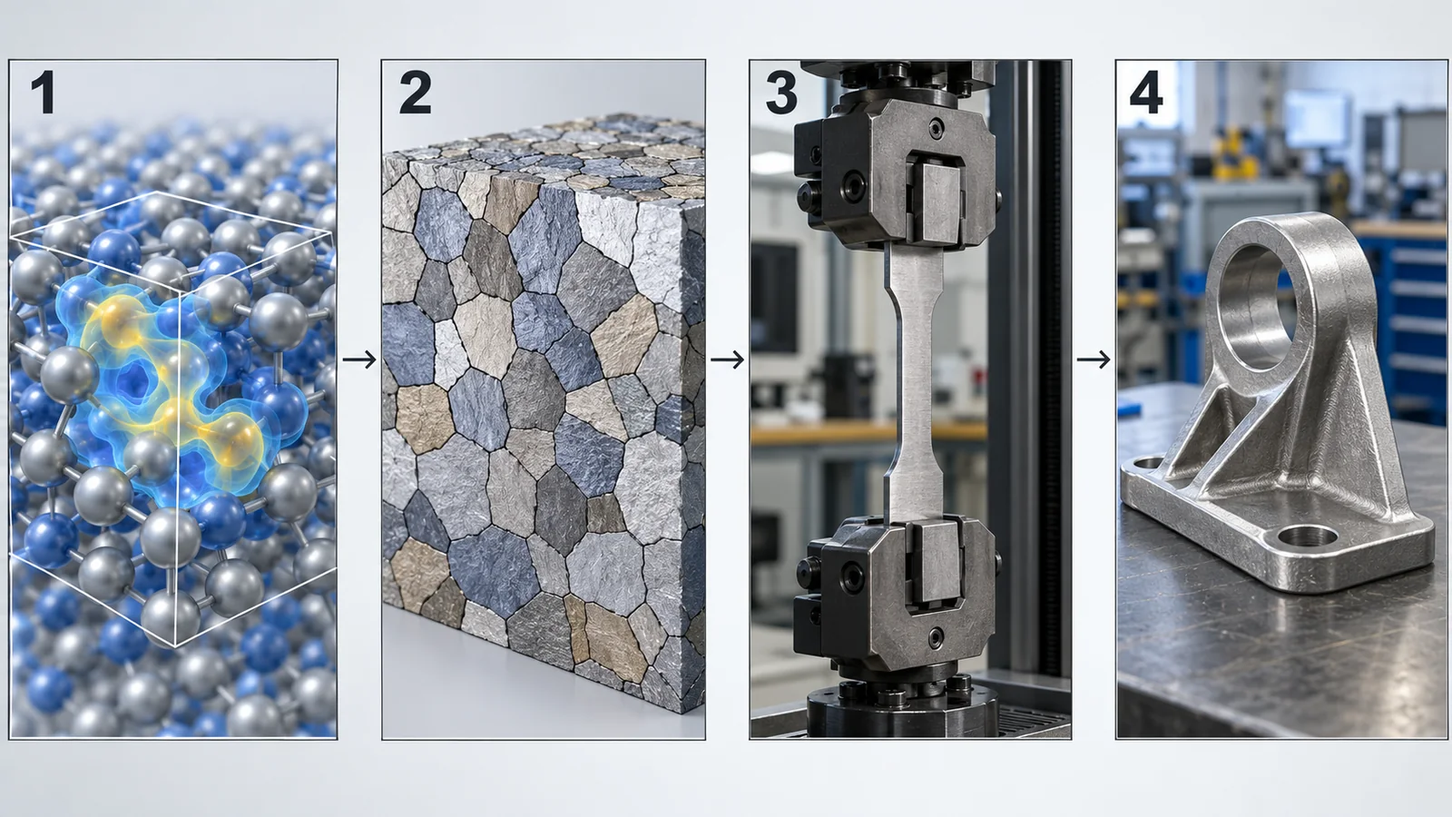
The properties of a component are set by phenomena at far smaller scales: the microstructure inside it, the motion of atoms, the behaviour of electrons. Yet no computer can calculate everything from the atoms up. So multiscale simulation links calculations at different scales: electrons → atoms → microstructure → component. A digital twin, in turn, is the idea of keeping a computational model linked to the real thing through data. Checking official documents and papers, this article sorts out the types of linkage, how errors propagate (our own calculation), what a digital twin means, and the limits when it is applied to materials.
- The short version, what to know first, and where this fits in the series
- What "scale" means: electrons, atoms, microstructure, components
- Why we cannot compute everything at once
- Types of linkage: pass values, go back and forth, solve together
- How errors below propagate above
- What is a digital twin?
- Digital twins of materials, and their limits
- Checking whether a result can be trusted
- A materials engineer's view
- Limits, what we could not confirm, and a summary
- How to read the yardsticks and standards
- Glossary
- References
- Claim-to-source audit
Sourced = stated in a published source (linked)
Our calculation = a value computed in this article from the stated assumptions
Not yet confirmed = plans, targets, drafts, work in progress, outlooks: not settled
Our own reading for materials engineers is marked as commentary. Inference is shown in bold.
1. The short version, what to know first, and where this fits in the series
- Multiscale simulation is the idea of "linking" calculations at levels of different size: electrons, atoms, microstructure and components. Linkage comes in three kinds: linking, which hands the results below to the level above; iterative coupling, which goes back and forth until convergence; and tight coupling, which solves everything at once as a single system Sourced[Ref. 1]
- When scales are linked, a small error at a lower level can swell at a higher level. In our calculation, a 0.05 eV error in an activation barrier changes a rate by about 6.9 times at 300 K Our calculation
- A digital twin is not simply a simulation. The National Academies report says "a digital twin is more than just simulation and modeling", and names the bidirectional interaction with the physical counterpart (updating by data and decision-making) as a key element Sourced[Ref. 19]. For materials there is the added difficulty that the state (the microstructure) cannot be seen directly (commentary)
The prerequisite is that the methods "that compute the motion of atoms (molecular dynamics)" and "that compute from the behaviour of electrons (DFT)" each handle a different size and time (see our explainers on molecular dynamics and on density functional theory). This article is readable on its own.
The ideas shared across this series: searching for materials is looking for buried treasure on a vast map; computation "proposes candidates quickly and cheaply", experiment "checks whether it is really so", and AI "narrows where to look". This article is about linking calculations to each other and linking calculation to the real thing.
We suggest reading it after our explainers on molecular dynamics and on machine-learning interatomic potentials (the atomic scale). How far a linked result can be trusted is covered in our explainers on uncertainty and applicability domains and on reading the evaluation and reproducibility of MI results. National and institutional plans are in our explainer on MI strategies and data infrastructure, and loops with experiment follow in our explainers on closed-loop optimization and self-driving laboratories.
2. What "scale" means: electrons, atoms, microstructure, components
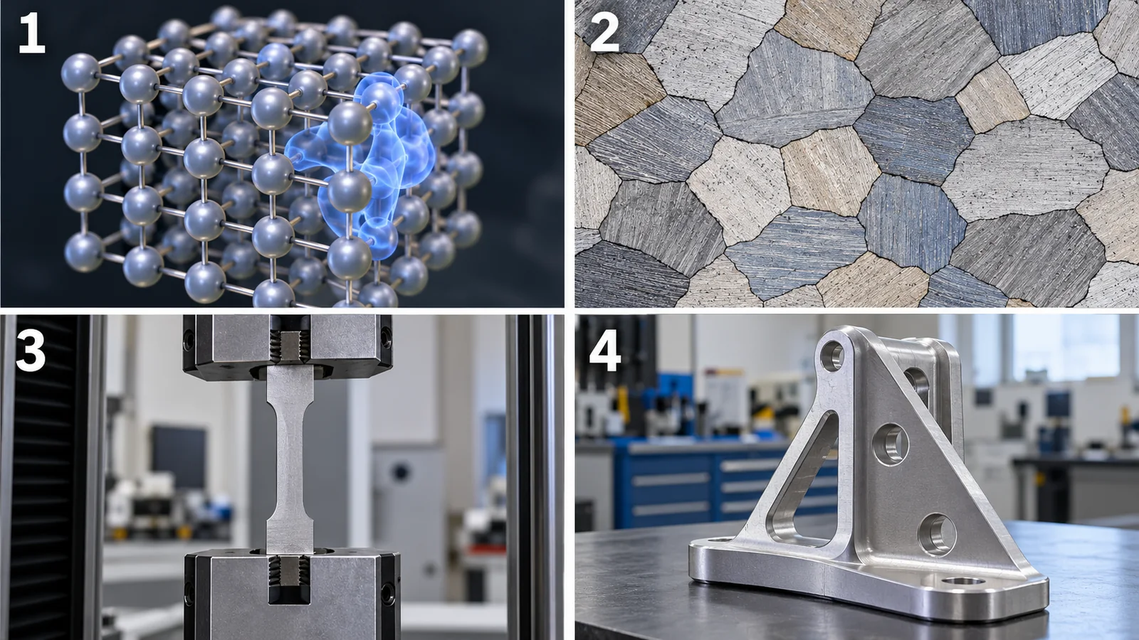
Even for the same metal part, a different size of view shows a different thing: the cloud of electrons, the arrangement of atoms, the pattern of grains (clusters of small crystals), and the shape of the whole part. At each level, the tools for calculation and the size and time that can be handled are different.
A document of the European standards body CEN (CEN Workshop Agreement 17284, April 2018) first divides materials models into four by the "entity" the model describes: electron entity, atom entity, mesoscopic entity (a set of bound atoms: a molecule, bead, grain and so on) and continuum volume entity Sourced[Ref. 1]. It also says that any material can be described by any of the entity types.
View original SVG, values and sources
Original SVG reference: Concept diagram (vector drawing). Four levels: electrons → atoms → microstructure → component. The four "entities" come from CEN CWA 17284. The scales are conceptual, not strict ranges for each method.
- Electrons: first-principles calculation (DFT) gives the energy surface and forces. What it passes to the level below is how the forces between atoms are set (the potential)
- Atoms: molecular dynamics computes diffusion coefficients, interface energies, elastic constants, thermal conductivity and so on (see our explainer on molecular dynamics)
- Microstructure (mesoscale): it handles grains and clusters of molecules. The phase-field method deals with the evolution of microstructure, and Chen (2002) wrote a review of it Sourced[Ref. 10]. There are also methods for the motion of dislocations (line defects in a crystal). Thermodynamic calculation (the CALPHAD method) is used at this level too (a history of CALPHAD is given by Spencer, 2008) [Ref. 11]
- Component: the finite-element method and similar tools compute deformation, heat and current in a part. This corresponds to the "continuum volume entity" in the CEN document
A higher level does not hold the fine detail of the level below. In a component calculation, for example, individual grains are not drawn; a value such as "on average, the elastic modulus of this material is this" is used. Condensing the fine detail of a lower level into an averaged value and passing it up is called homogenization (upscaling). Conversely, bringing the forces on the component down to a lower level to see local stresses is called localization. Kalidindi et al. (2022) say that, for a digital twin of a material, surrogate models at each scale are used in a framework of homogenization and localization Sourced[Ref. 12].
3. Why we cannot compute everything at once
You may think: "Then just compute the whole part from the atoms." Let us estimate the amount of calculation. As seen in our explainer on molecular dynamics, advancing 1 second in steps of 1 fs (10⁻¹⁵ s) takes 10¹⁵ steps, and 1 mm³ of iron holds about 8.5×10¹⁹ atoms Our calculation.
- The records: Germann and Kadau (2008) report MD of one trillion atoms, and Jia et al. (2020) report, with a machine-learning potential and a dedicated code, more than 100 million atoms advanced by more than 1 ns per day Sourced[Refs. 17, 16]. One trillion atoms of iron fill a cube only about 2.3 μm on a side Our calculation
- The estimate: for 1 mm³ and 1 second with all atoms, atoms × steps is about 8.5×10³⁴. Dividing by the throughput of Jia et al. (at least about 10¹⁴ per day) gives about 8.5×10²⁰ days, or about 2×10¹⁸ years (an upper bound) Our calculation. Even the record runs are off by a huge number of orders of magnitude
So instead of computing everything at once with atoms, we need to take out "only the necessary information" at each level and pass it up. The 2013 Nobel Prize in Chemistry went to Karplus, Levitt and Warshel "for the development of multiscale models for complex chemical systems". Their achievement is described as making Newton's classical physics work side by side with quantum physics Sourced[Ref. 2].
4. Types of linkage: pass values, go back and forth, solve together
There are three main types of linkage. The CEN document defines the terms as follows (3.14 to 3.16) Sourced[Ref. 1].
- Linking: the output of model A becomes the input of model B. One-way, with an open flow. The most common form. For example: from DFT values build a potential for molecular dynamics, and pass the diffusion coefficient from molecular dynamics to a microstructure calculation (commentary)
- Iterative coupling: A and B take each other's outputs as inputs and go back and forth until they converge. The flow is closed
- Tight coupling: the equations of A and B are collected and solved at once as a single system of equations. The result comes out as one output
The standard examples of "at once" are methods that couple in space.
- QM/MM: a method that treats only the centre where a reaction occurs with quantum mechanics and the surroundings with classical mechanics. Warshel and Levitt (1976) used it in a theoretical study of an enzyme (lysozyme) reaction [Ref. 3]. It is part of the work honoured by the 2013 Nobel Prize in Chemistry [Ref. 2] Sourced
- Coupling atoms and a continuum: Rudd and Broughton (1999) report, for MEMS (tiny mechanical parts) resonators, a method in which the central region moves millions of individual atoms, the large peripheral regions are computed with finite elements, and the two methods run concurrently and pass information back and forth. They say atoms are needed in regions of strongly anharmonic forces, of large surface-to-volume ratio, and where friction due to defects is expected Sourced[Ref. 4]. The paper by Broughton et al. (1999) deals with coupling finite elements, molecular dynamics and tight-binding electronic structure [Ref. 5]
- A case of handing values up in stages and confirming by experiment: Bulatov et al. (2006) predicted the existence of three-dislocation entanglements (multi-junctions) with dislocation dynamics and atomistic simulation, and confirmed them by transmission electron microscopy of molybdenum Sourced[Ref. 6]. Calculations at several scales were combined and tested by experiment
There is also coarse-graining, which lumps several atoms into one ball to handle larger systems. Examples are entangled polymers (Kremer and Grest, 1990) and a coarse-grained force field for biomolecules (Marrink et al., 2007, MARTINI), and there is a review of multiscale simulation in polymer science (Kremer and Müller-Plathe, 2002) Sourced[Refs. 7, 9, 8].
In materials, the idea of building calculation into design and manufacturing is called ICME (Integrated Computational Materials Engineering). A 2008 report of the U.S. National Research Council places ICME as "an emerging discipline that can accelerate materials development and unify design and manufacturing" Sourced[Ref. 13]. As an industrial example there is a paper whose subject is applying ICME to cast aluminium parts (Allison et al., 2006) [Refs. 14, 15]. We did not check the figures for individual effects.
5. How errors below propagate above
Linking brings a new problem: errors at a lower level propagate to the level above. There are two typical ways.
- Exponential amplification: the speed of diffusion or reaction is set by exp(−E/k_B T) for a barrier E. If the barrier is off by ΔE, the rate ratio is exp(ΔE/k_B T). With ΔE = 0.05 eV, it is about 6.9 times at 300 K, about 2.6 times at 600 K and about 1.8 times at 1000 K. With ΔE = 0.1 eV, about 48 times at 300 K Our calculation. A "small" energy error at a lower level (DFT) becomes a large error at the level above (rate). It is most marked at low temperatures
- Accumulation over stages: suppose each stage is "within a factor of 2 at 95%". If the errors are independent, four stages widen to about 4 times overall (2^√4). If they all lean the same way, 16 times (2⁴) Our calculation. In a real chain errors can be correlated, for example when the same DFT bias is carried up to higher levels (commentary)
It is the opposite. The accuracy of the linked whole is set by the weakest stage and by how errors propagate. Even if the bottom layer uses precise DFT, that accuracy does not reach the top if a middle model is coarse. And, as Fig. 5 shows, errors are amplified and accumulate. A linked result is checked by verifying each stage and comparing the whole with measurement (chapter 8) (commentary).
6. What is a digital twin?
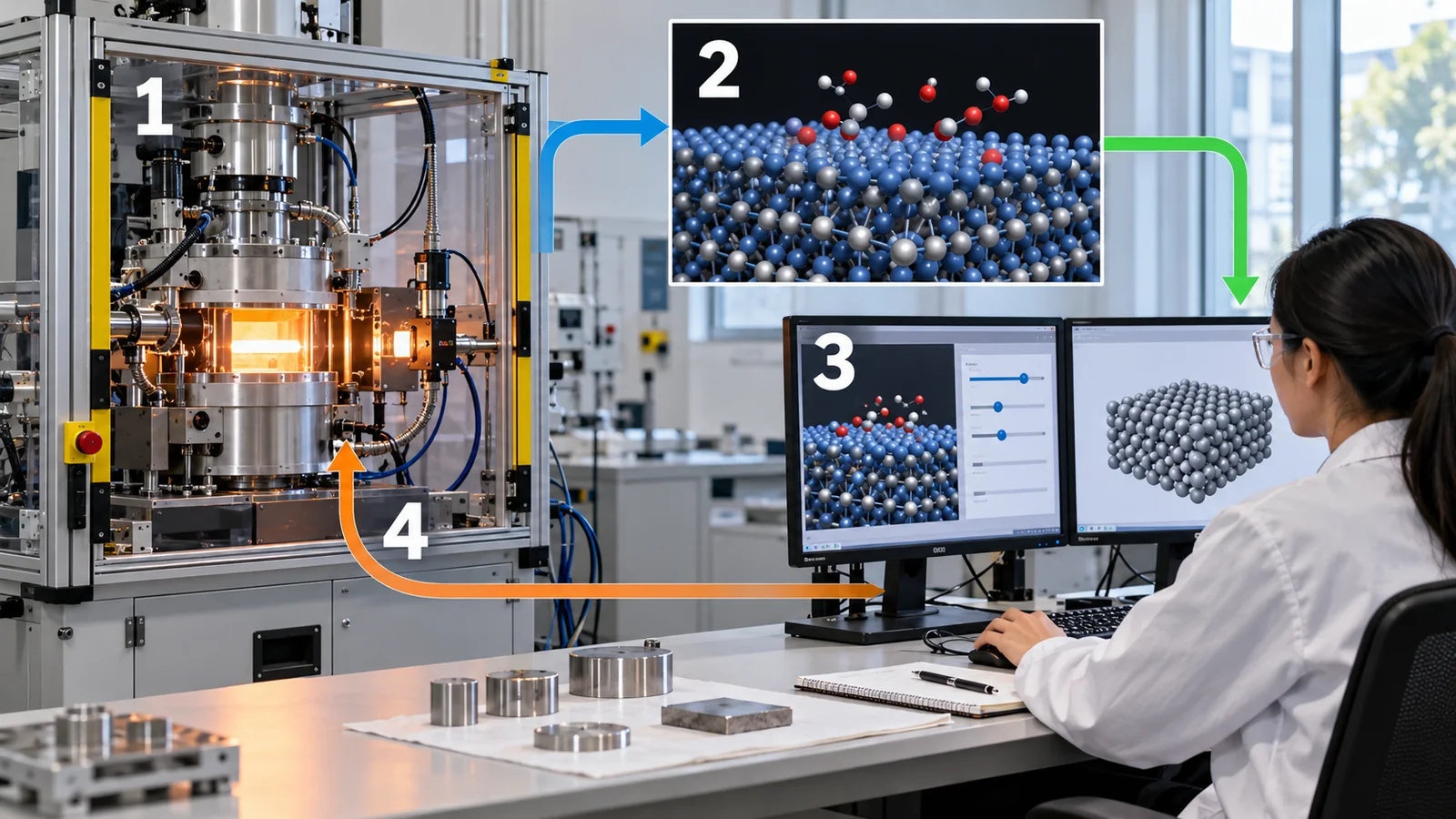
Next, the digital twin. As the name "twin" says, it is the idea that the real thing (the physical counterpart) and a computational model (the virtual counterpart) are kept connected through data. We check the definitions in official documents.
- NASA (2012): Glaessgen and Stargel say that certification and sustainment of future NASA and U.S. Air Force vehicles rely largely on statistical distributions of material properties, heuristic design philosophies, physical testing and assumed similitude between testing and operating conditions, and that these will be unable to meet extreme requirements; they propose the digital twin as the shift. The digital twin integrates ultra-high-fidelity simulation with the vehicle's health-management system, maintenance history and all available historical and fleet data to mirror the life of its flying twin Sourced[Ref. 18]
- National Academies (2024): it defines a digital twin as "a set of virtual information constructs that mimics the structure, context, and behavior of a natural, engineered, or social system (or system-of-systems), is dynamically updated with data from its physical twin, has a predictive capability, and informs decisions that realize value. The bidirectional interaction between the virtual and the physical is central" (adapted from a definition by AIAA). It also states that "a digital twin is more than just simulation and modeling" (Finding 2-1) Sourced[Ref. 19]
- International standards: ISO/IEC 30173:2023 (Digital twin — Concepts and terminology) sets terms and concepts for the digital twin (system context, life cycle, types, functional view, stakeholders) and was published in November 2023. ISO 23247-1:2021 gives an overview and general principles of a digital twin framework for manufacturing (terms and requirements) and was published in October 2021 Sourced[Refs. 23, 22]. The texts are paid, and we did not check the requirements
View original SVG, values and sources
Original SVG reference: Concept diagram (vector drawing). Left: the structure of a digital twin (following the NASEM account). Right: three levels of integration (the classification of Kritzinger et al.; the account follows the summary by Barbie and Hasselbring).
Kritzinger et al. (2018) surveyed the manufacturing literature, found that there is no common understanding of the term digital twin, and distinguished the digital model, digital shadow and digital twin by the level of integration. They report that literature on the most advanced stage, the digital twin, is scarce Sourced[Ref. 20]. As summarised by Barbie and Hasselbring (2024), the three levels are: digital model: no automated data exchange; digital shadow: an automated one-way flow from physical to virtual; digital twin: automated in both directions [Ref. 21]. The same paper also reports Grieves's criticism of this classification, and the view that ISO 23247 does not mention bidirectional communication and so, on this definition, describes only a digital shadow [Ref. 21]. This article simply shows that definitions vary.
The National Academies report says that a digital twin is more than simulation and modeling; its elements include bidirectional interaction with the physical counterpart (updating of the model by sensors and so on, and control and decision-making) [Ref. 19]. If a high-precision model, once built, is used only for design studies and is not updated with data from the real thing, it is a "digital model" (the classification of Kritzinger et al.). Judge by the direction, frequency and use of the updates, not by the name (commentary).
7. Digital twins of materials, and their limits
Digital twins of aircraft and plants have many quantities that sensors can measure (strain, temperature, vibration). How, then, is a digital twin of the material itself thought of?
- The idea: Kalidindi et al. (2022) regard the material itself as a highly complex multiscale physical system. Its form (details of the hierarchical structure) and function (response to external stimuli, that is, properties) are captured in a digital twin. They argue that the digital twin can represent how structure, process and performance of the material evolve over time, given both process history and in-service environment. The form is captured with n-point spatial correlations and the function with homogenization and localization surrogate models, calibrated to experimental and physics-based simulation data Sourced[Ref. 12]
- Standing: the paper sets out foundational concepts and a framework; it is not a demonstration on a real material (our reading)
- What is hard: (1) The state (microstructure and so on) often cannot be seen directly in service and is inferred from what can be measured. (2) Each part has a different processing history, so each individual needs its own updating. (3) Errors of the models linking the scales propagate to the whole (Fig. 5). These are our own organisation (commentary)
The National Academies report says the virtual side of a digital twin should be built at a fidelity and resolution that is "fit for purpose", matched to the decision to be made and the computing resources (Conclusion 3-1), and that it may mix high-fidelity, simplified and surrogate models Sourced[Ref. 19]. For materials as well, what you want to decide sets the scale and accuracy needed (commentary).
8. Checking whether a result can be trusted
For linked calculations and for digital twins alike, the work of checking whether a result can be trusted makes up half of the job. The National Academies report says that verification, validation and uncertainty quantification (VVUQ) have a role in all elements of a digital twin. On the virtual side, verification and validation build trustworthiness, and uncertainty quantification gives a measure of the quality of prediction Sourced[Ref. 19]. It also says that changes in the physical counterpart, in data collection, in the distribution of data, in the prediction or decision tasks and in the models all bear on VVUQ [Ref. 19].
- Verification: are the equations solved correctly (code errors, numerical error, time step and so on)? Checking energy conservation, in our explainer on molecular dynamics, is one example
- Validation: are these the right equations and model? Compare with measurement of the same quantity under the same conditions
- Uncertainty quantification (UQ): how much do scatter in the inputs and the model affect the prediction? Give the prediction with a range
- A standard: ASME V&V 10-2019 is a standard for verification and validation in computational solid mechanics; it was reaffirmed in 2025 (R2025) and remains in effect Sourced[Ref. 24]. It bears on checking the continuum stage of a linked chain. The text is paid, and we did not check the requirements
9. A materials engineer's view
For the calculation at each stage, tabulate what goes in and what comes out. For example: "DFT: structure → activation barrier", "molecular dynamics: temperature and barrier → diffusion coefficient", "microstructure calculation: diffusion coefficient and interface energy → change of microstructure", "component calculation: effective elastic modulus → stress". The CEN document gives a documentation format (MODA) with items for the use case, model, time step, software and the input received from the earlier stage [Ref. 1]. Recording which value came from which stage lets you trace later where something is suspect.
As Fig. 5 shows, quantities that act exponentially (activation barriers, interface energies) turn a small error into a large difference in the result. First identify the input that matters most for the result, check it by measurement (for example, find the activation energy of diffusion from measurements at several temperatures) and compare it with the model value. If you design experiments (controls, reproducibility, lot-to-lot differences) starting from the inputs that matter, you waste less (commentary).
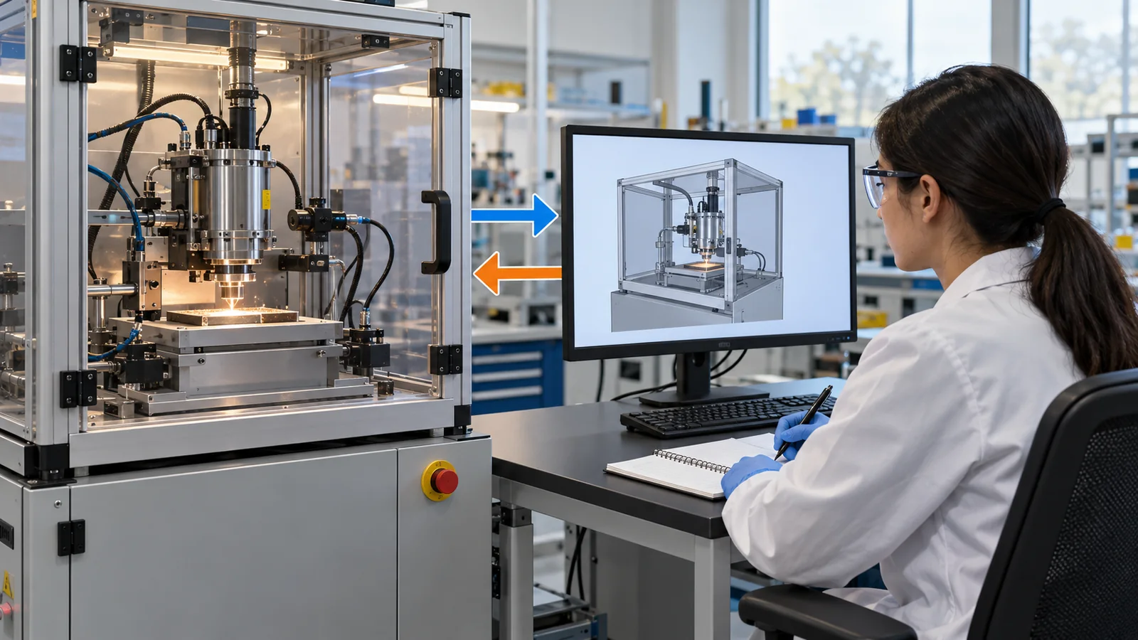
Rather than posing grandly as a "digital twin", it is realistic to start in a small area, in a form that really can be updated. For example, in one of your own processes (heat treatment, forming), link what you can measure (temperature history, strain, hardness) with what you compute (microstructure, strength), and update the model parameters with the measurements. The frequency and direction of the update separate a "model", a "shadow" and a "twin" (Fig. 6). A mechanism for recording the history of each individual (lot, processing conditions) is the foundation (commentary).
To update a model you need data. Beyond measured values, attach the sample's manufacturing route, thermal history, assay values of the composition, the measurement conditions and equipment, and the lot, and keep them in fixed fields, not in free-text spreadsheet cells. Record experiments that did not work and the reasons for outliers too. The conditions under which a model went wrong are clues to the edge of its range of application.
10. Limits, what we could not confirm, and a summary
- Multiscale simulation links electrons, atoms, microstructure and components. The types of linkage are linking (one-way), iterative coupling (back and forth) and tight coupling (at once). QM/MM and the coupling of atoms with a continuum are examples of concurrent coupling Sourced
- We link because we cannot compute everything with atoms. Simulating 1 mm³ for 1 second with every atom would take about 2×10¹⁸ years even at the throughput of the record runs Our calculation
- Linking makes errors propagate. A 0.05 eV error in a barrier becomes about 6.9 times in rate at 300 K, and even if each stage is "within a factor of 2", four stages can widen to about 4 to 16 times Our calculation
- A digital twin is not a simulation by itself; its elements include bidirectional interaction with the physical counterpart. For materials, the microstructure cannot be seen directly and each individual has a different history. Verification, validation and uncertainty quantification are needed in every element Sourced
What we could not confirm
- The scales (length and time) in Fig. 2 are a conceptual organisation; we did not check the numbers in individual literature
- Warshel and Levitt (1976), Broughton et al. (1999), Allison et al. (2006), Kremer and Müller-Plathe (2002), Chen (2002) and Spencer (2008) were handled within the range of the title and the publicly available abstract or description. We did not check details of the full texts
- The explanations of the CALPHAD and phase-field methods are commentary based on general understanding; we did not check the full texts of individual literature
- We could not check the text of the classification by Kritzinger et al., and the content of the three levels follows the summary by Barbie and Hasselbring (2024)
- The calculation in Fig. 5 is an example based on assumptions (Arrhenius type, independent log-normal distributions) and does not estimate the errors of any real chain
- The texts (requirements) of ISO 23247-1, ISO/IEC 30173 and ASME V&V 10 are paid and we did not check them. Titles, status and scope were checked on the official pages
- We could not find an international standard for digital twins of materials. We also did not check the number and maturity of demonstrations of digital twins in materials
11. How to read the yardsticks and standards
The yardsticks for multiscale simulation and digital twins are, first, verification of the calculation at each stage (are the equations solved correctly), then comparison with measurement (validation), uncertainty (predictions with a range) and fitness for purpose. What the yardsticks do not measure is the behaviour of the whole linked chain under unseen conditions. Checked on 22 October 2026.
| Item | Representative benchmarks and methods (name, source) | Standards and guidance (ISO/IEC, NIST, CEN, etc.) | Reading notes |
|---|---|---|---|
| Terminology and describing linkage | CEN CWA 17284: classification by entity (electron, atom, mesoscopic, continuum). Definitions of linking, iterative coupling and tight coupling. MODA (documentation template) [Ref. 1] Sourced | CWA 17284:2018 (CEN Workshop Agreement, April 2018). Not an official standard. It covers physics-based models and excludes data-based models [Ref. 1] Sourced | A documentation format; it does not guarantee that the result is correct |
| Terminology and frameworks for digital twins | NASEM (2024): definition and conclusions [Ref. 19]. The three levels of Kritzinger et al. [Ref. 20] Sourced | ISO/IEC 30173:2023 (terminology and concepts, published November 2023) [Ref. 23]. ISO 23247-1:2021 (framework for manufacturing, overview and general principles, published October 2021) [Ref. 22] Sourced | The texts are paid and the requirements were not checked. One view is that ISO 23247 does not mention bidirectional communication (Barbie and Hasselbring). Definitions vary |
| Verification, validation and uncertainty quantification (VVUQ) | NASEM (2024): VVUQ is needed in all elements of a digital twin [Ref. 19] Sourced | ASME V&V 10-2019 (R2025): a standard for V&V in computational solid mechanics [Ref. 24] Sourced | The standard targets the continuum (solid mechanics) stage. We could not confirm V&V standards for the electron and atom stages |
| How errors propagate through a linked chain | Our calculation (Fig. 5): amplification of a barrier error and accumulation over stages [this article] Our calculation | Could not be confirmed | An example based on assumptions. For your own chain, estimate the correlations and how strongly each input acts |
| Industrial use and policy standing | NRC (2008): the standing of ICME [Ref. 13] Sourced | Could not be confirmed (an international standard for digital twins of materials) | The report is policy and recommendation, not a standard. We did not check figures for its effect |
The organisation of the table is Our calculation (our arrangement). Numbers, titles and status were checked on the official pages of ISO, ASME, CEN and NASEM (checked on 22 October 2026). Because the texts of standards are paid, we limit ourselves to titles and scope and do not write requirements. We did not confirm any applicable ASTM standard within the scope of this article.
Reading notes (for materials engineers)
- Judge by content, not by name: if something calls itself a "digital twin" but the updates are one-way or manual, it is a shadow or a model. Check the effect of adoption by the frequency and direction of updates, not by the name
- Prediction versus experimental confirmation: the prediction of a linked calculation can be used for decisions only after verification of each stage and comparison of the whole with measurement (the case of Bulatov et al. is one in which a calculated prediction was confirmed by experiment) [Ref. 6]
- Are standards and guidance recommended or required? The CWA is not an official standard; ISO 30173 and 23247 are terminology and frameworks; ASME V&V 10 is a voluntary standard. All of them generally have binding force only when a contract or law cites them (commentary)
- Plan versus achievement: introduction plans for digital twins and the visions of countries and companies are targets. Check whether updating actually runs
12. Glossary
- Multiscale simulation
- The idea of linking calculations at levels of different size, such as electrons, atoms, microstructure and components.
- Entity
- In the CEN document, the unit a model describes. Four kinds: electron, atom, mesoscopic and continuum.
- Mesoscale
- A size between atoms and components (grains, clusters of molecules and so on).
- Continuum
- A view that treats the material as continuous matter without dividing it into atoms. Finite elements and so on.
- Linking
- One-way coupling in which the output of model A becomes the input of B.
- Iterative coupling
- Coupling in which two models take each other's outputs as inputs and go back and forth until convergence.
- Tight coupling
- Coupling in which the equations of two models are solved at once as a single system.
- QM/MM
- A method that treats the centre with quantum mechanics (QM) and the surroundings with classical mechanics (MM).
- Homogenization (upscaling)
- Condensing the fine detail of a lower level into averaged values and passing them to the level above.
- Localization
- Passing the conditions on a component down to a lower level to see local stresses and so on.
- Coarse-graining
- Lumping several atoms into one ball to handle larger systems.
- Phase-field method
- A method that treats the evolution of microstructure as continuous fields.
- CALPHAD
- A method that uses thermodynamic databases to compute phase stability and so on.
- ICME
- Integrated computational materials engineering. The idea of building calculation into the development, design and manufacturing of materials.
- Digital twin
- The idea that a physical counterpart and a virtual model stay connected by data in both directions.
- Digital model / shadow / twin
- Three levels by the presence and direction of automated data exchange (the classification of Kritzinger et al.).
- Data assimilation
- Updating the state or parameters of a model with observed data.
- Surrogate model
- A simple model (machine learning and so on) that approximates a heavy calculation quickly.
- Verification / validation (V&V)
- Are the equations solved correctly / are they the right equations and model?
- Uncertainty quantification (UQ)
- Quantifying how scatter in the inputs and the model affects the prediction. VVUQ is the collective term for the three.
- Fit for purpose
- Having accuracy and resolution that suffice for the decision to be made.
- MODA
- Materials modelling data. The documentation template for a simulation given in the CEN document.
13. References
- CEN (European Committee for Standardization) "CEN Workshop Agreement CWA 17284:2018, Materials modelling - Terminology, classification and metadata" (2018) — www.cencenelec.eu/media/CEN-CENELEC/CWAs/RI/cwa17284_2018.pdf
- The Royal Swedish Academy of Sciences "The Nobel Prize in Chemistry 2013, press release (9 October 2013)" — www.nobelprize.org/prizes/chemistry/2013/press-release/
- Warshel A., Levitt M. "Theoretical studies of enzymic reactions: Dielectric, electrostatic and steric stabilization of the carbonium ion in the reaction of lysozyme", J. Mol. Biol. 103, 227–249 (1976), DOI 10.1016/0022-2836(76)90311-9 — doi.org/10.1016/0022-2836(76)90311-9
- Rudd R. E., Broughton J. Q. "Coupling of length scales and atomistic simulation of MEMS resonators", SPIE Proceedings 3680, 104 (arXiv:cond-mat/9812232) (1999), DOI 10.1117/12.341254 — doi.org/10.1117/12.341254
- Broughton J. Q., Abraham F. F., Bernstein N., Kaxiras E. "Concurrent coupling of length scales: Methodology and application", Phys. Rev. B 60, 2391–2403 (1999), DOI 10.1103/PhysRevB.60.2391 — doi.org/10.1103/PhysRevB.60.2391
- Bulatov V. V. et al. "Dislocation multi-junctions and strain hardening", Nature 440, 1174–1178 (2006), DOI 10.1038/nature04658 — doi.org/10.1038/nature04658
- Kremer K., Grest G. S. "Dynamics of entangled linear polymer melts: A molecular-dynamics simulation", J. Chem. Phys. 92, 5057–5086 (1990), DOI 10.1063/1.458541 — doi.org/10.1063/1.458541
- Kremer K., Müller-Plathe F. "Multiscale simulation in polymer science", Mol. Simul. 28, 729–750 (2002), DOI 10.1080/0892702021000002458 — doi.org/10.1080/0892702021000002458
- Marrink S. J. et al. "The MARTINI Force Field: Coarse Grained Model for Biomolecular Simulations", J. Phys. Chem. B 111, 7812–7824 (2007), DOI 10.1021/jp071097f — doi.org/10.1021/jp071097f
- Chen L.-Q. "Phase-Field Models for Microstructure Evolution", Annu. Rev. Mater. Res. 32, 113–140 (2002), DOI 10.1146/annurev.matsci.32.112001.132041 — doi.org/10.1146/annurev.matsci.32.112001.132041
- Spencer P. J. "A brief history of CALPHAD", Calphad 32, 1–8 (2008), DOI 10.1016/j.calphad.2007.10.001 — doi.org/10.1016/j.calphad.2007.10.001
- Kalidindi S. R., Buzzy M., Boyce B. L., Dingreville R. "Digital Twins for Materials", Front. Mater. 9, 818535 (2022), DOI 10.3389/fmats.2022.818535 — doi.org/10.3389/fmats.2022.818535
- National Research Council (U.S.) "Integrated Computational Materials Engineering: A Transformational Discipline for Improved Competitiveness and National Security", The National Academies Press (2008), DOI 10.17226/12199 — doi.org/10.17226/12199
- Allison J., Backman D., Christodoulou L. "Integrated computational materials engineering: A new paradigm for the global materials profession", JOM 58 (11), 25–27 (2006), DOI 10.1007/s11837-006-0223-5 — doi.org/10.1007/s11837-006-0223-5
- Allison J. et al. "Virtual aluminum castings: An industrial application of ICME", JOM 58 (11), 28–35 (2006), DOI 10.1007/s11837-006-0224-4 — doi.org/10.1007/s11837-006-0224-4
- Jia W. et al. "Pushing the limit of molecular dynamics with ab initio accuracy to 100 million atoms with machine learning", arXiv:2005.00223 (SC20) (2020) — arxiv.org/abs/2005.00223
- Germann T. C., Kadau K. "Trillion-atom molecular dynamics becomes a reality", Int. J. Mod. Phys. C 19, 1315–1319 (2008), DOI 10.1142/S0129183108012911 — doi.org/10.1142/S0129183108012911
- Glaessgen E., Stargel D. "The Digital Twin Paradigm for Future NASA and U.S. Air Force Vehicles", NASA Technical Reports Server 20120008178 (AIAA 2012-1818) (2012) — ntrs.nasa.gov/citations/20120008178
- National Academies of Sciences, Engineering, and Medicine "Foundational Research Gaps and Future Directions for Digital Twins (Summary chapter)", The National Academies Press (2024) — nap.nationalacademies.org/read/26894/chapter/2
- Kritzinger W. et al. "Digital Twin in manufacturing: A categorical literature review and classification", IFAC-PapersOnLine 51 (11), 1016–1022 (2018), DOI 10.1016/j.ifacol.2018.08.474 — doi.org/10.1016/j.ifacol.2018.08.474
- Barbie A., Hasselbring W. "From Digital Twins to Digital Twin Prototypes: Concepts, Formalization, and Applications", IEEE Access arXiv:2401.07985 (2024), DOI 10.1109/ACCESS.2024.3406510 — doi.org/10.1109/ACCESS.2024.3406510
- ISO ISO 23247-1:2021 Automation systems and integration — Digital twin framework for manufacturing — Part 1: Overview and general principles (page checked 22 October 2026) (2021) — www.iso.org/standard/75066.html
- ISO/IEC ISO/IEC 30173:2023 Digital twin — Concepts and terminology (page checked 22 October 2026) (2023) — www.iso.org/standard/81442.html
- ASME V&V 10-2019 (R2025) Standard for Verification and Validation in Computational Solid Mechanics (page checked 22 October 2026) (2019) — www.asme.org/codes-standards/find-codes-standards/standard-for-verification-and-validation-in-computational-solid-mechanics
14. Claim-to-source audit
| Claim in the text | Basis | Type |
|---|---|---|
| CEN CWA 17284:2018 (April 2018): models classified by entity (electron, atom, mesoscopic, continuum volume). Definitions of linking, iterative coupling and tight coupling (3.14 to 3.16). MODA is a documentation template. It covers physics-based models. Not an official standard | Reference 1 https://www.cencenelec.eu/media/CEN-CENELEC/CWAs/RI/cwa17284_2018.pdf | Sourced |
| Our calculation: 1 s is 10¹⁵ steps of 1 fs. 1 mm³ of iron holds about 8.5×10¹⁹ atoms, and 10¹² atoms fill a cube about 2.3 μm on a side (estimated from density 7.87 g/cm³ and molar mass 55.85 g/mol) | our calculation | Our calculation |
| The record runs: one trillion Lennard-Jones particles by Germann and Kadau (2008); more than 10⁸ atoms at more than 1 ns per day by Jia et al. (2020, Summit) | Reference 17 https://doi.org/10.1142/S0129183108012911 Reference 16 https://arxiv.org/abs/2005.00223 | Sourced |
| Estimate for 1 mm³ and 1 s with every atom: atoms × steps about 8.5×10³⁴; at the throughput of Jia et al. (at least about 10¹⁴ per day) about 8.5×10²⁰ days, about 2×10¹⁸ years (an upper bound) | our calculation (the value of Jia et al. is a lower bound, so the number of years is an upper bound) | Our calculation |
| Nobel Prize in Chemistry 2013: development of multiscale models for complex chemical systems (Karplus, Levitt, Warshel). Classical and quantum physics made to work side by side | Reference 2 https://www.nobelprize.org/prizes/chemistry/2013/press-release/ | Sourced |
| QM/MM: Warshel and Levitt (1976), a theoretical study of an enzyme (lysozyme) reaction | Reference 3 https://doi.org/10.1016/0022-2836(76)90311-9 | Sourced |
| Rudd and Broughton: in MEMS resonators, millions of atoms in the centre and finite elements in the periphery; the two methods run concurrently and pass information back and forth. Broughton et al.: concurrent coupling of finite elements, molecular dynamics and tight binding (title) | Reference 4 https://doi.org/10.1117/12.341254 Reference 5 https://doi.org/10.1103/PhysRevB.60.2391 | Sourced |
| Bulatov et al.: dislocation multi-junctions predicted with dislocation dynamics and atomistic simulation and confirmed by transmission electron microscopy of molybdenum | Reference 6 https://doi.org/10.1038/nature04658 | Sourced |
| Coarse-graining examples: Kremer and Grest (1990, entangled polymer melts), Marrink et al. (2007, MARTINI), Kremer and Müller-Plathe (2002, multiscale simulation in polymer science) | Reference 7 https://doi.org/10.1063/1.458541 Reference 9 https://doi.org/10.1021/jp071097f Reference 8 https://doi.org/10.1080/0892702021000002458 | Sourced |
| A review of the phase-field method (Chen, 2002). A history of CALPHAD (Spencer, 2008). The explanations of how the two methods work are commentary based on general understanding | Reference 10 https://doi.org/10.1146/annurev.matsci.32.112001.132041 Reference 11 https://doi.org/10.1016/j.calphad.2007.10.001 | Sourced |
| Kalidindi et al. (2022): a framework for a digital twin of a material, regarding the material as a multiscale physical system and capturing form (n-point spatial correlations) and function (homogenization and localization surrogate models). Calibrated to experimental and physics-based simulation data | Reference 12 https://doi.org/10.3389/fmats.2022.818535 | Sourced |
| ICME: the NRC (2008) places it as an emerging discipline that can accelerate materials development and unify design and manufacturing. Allison et al. (2006): a new paradigm for ICME, and an application to cast aluminium parts (titles) | Reference 13 https://doi.org/10.17226/12199 Reference 14 https://doi.org/10.1007/s11837-006-0223-5 Reference 15 https://doi.org/10.1007/s11837-006-0224-4 | Sourced |
| Rate ratio exp(ΔE/k_B T) for an error ΔE in an activation barrier: 0.05 eV gives about 6.9 times at 300 K, 2.6 times at 600 K and 1.8 times at 1000 K; 0.1 eV at 300 K gives about 48 times (k_B = 8.617×10⁻⁵ eV/K). If each stage is within a factor of 2 at 95%, four stages give about 4 times if independent and 16 times if fully in the same direction (with assumptions) | our calculation (Arrhenius type and independent log-normal assumptions) | Our calculation |
| NASA (2012): certification and sustainment rely on statistical distributions of material properties, physical testing and so on; the digital twin integrates ultra-high-fidelity simulation with the vehicle health-management system, maintenance history and past data to mirror the life of its flying twin | Reference 18 https://ntrs.nasa.gov/citations/20120008178 | Sourced |
| National Academies (2024): the definition of a digital twin (bidirectional interaction is central), Finding 2-1 (more than simulation and modeling), Conclusion 3-1 (fit for purpose), VVUQ has a role in all elements | Reference 19 https://nap.nationalacademies.org/read/26894/chapter/2 | Sourced |
| Kritzinger et al. (2018): digital model, shadow and twin distinguished by level of integration; literature on the digital twin is scarce. The content of the three levels (presence and direction of automated data exchange), Grieves's criticism and the view on ISO 23247 follow the summary by Barbie and Hasselbring (2024) | Reference 20 https://doi.org/10.1016/j.ifacol.2018.08.474 Reference 21 https://doi.org/10.1109/ACCESS.2024.3406510 | Sourced |
| ISO/IEC 30173:2023 (November 2023, terminology and concepts for the digital twin) and ISO 23247-1:2021 (October 2021, overview and general principles of the framework for manufacturing). Texts are paid and were not checked | Reference 23 https://www.iso.org/standard/81442.html Reference 22 https://www.iso.org/standard/75066.html | Sourced |
| ASME V&V 10-2019 (R2025): a standard for verification and validation in computational solid mechanics. Reaffirmed in 2025 and in effect | Reference 24 https://www.asme.org/codes-standards/find-codes-standards/standard-for-verification-and-validation-in-computational-solid-mechanics | Sourced |
| A materials engineer's views (tabulating inputs and outputs, finding the inputs that matter, starting small, organising data). Linking homogenization, localization and fitness for purpose, and the list of what is hard for digital twins of materials, are commentary | commentary (our own view) | |
| We could not find an international standard for digital twins of materials, a literature source for the numbers in the scales of Fig. 2, or the number and maturity of demonstrations | our own check (could not be confirmed) |
Last updated: 22 October 2026. Sources are limited to primary material (papers, reports of NASA, the National Academies and the NRC, and official pages of CEN, ISO, ASME and the Nobel Prize). Numerical examples are our own calculations and do not show the errors of any real chain. We could not confirm the numerical scales in Fig. 2, some details of the full texts of papers, the text of the classification by Kritzinger et al., the texts (requirements) of the standards, or any international standard for digital twins of materials and the number of demonstrations, so we do not assert them. Figs. 2 to 8 are illustrative concept diagrams or drawings that include our calculations; Figs. 1 and 9 are AI-generated images (only the scene to be drawn is specified).