TECHNOLOGY EXPLAINER
AI Analysis of Spectra and Images
— how much of "reading the measured data" can be left to AI?
In a materials lab, someone reads measured data almost every day: an X-ray diffraction (XRD) waveform, a spectroscopy trace, an electron micrograph. A growing body of research asks AI, trained on past data, to help with that reading. But a figure such as "94% accuracy" can mean very different things depending on what data it was measured on, how the data were split, and what counted as the right answer. This article explains three jobs — identifying phases, classifying microstructures and removing noise — with diagrams and small calculations, and ends with how to read accuracy claims together with their conditions.
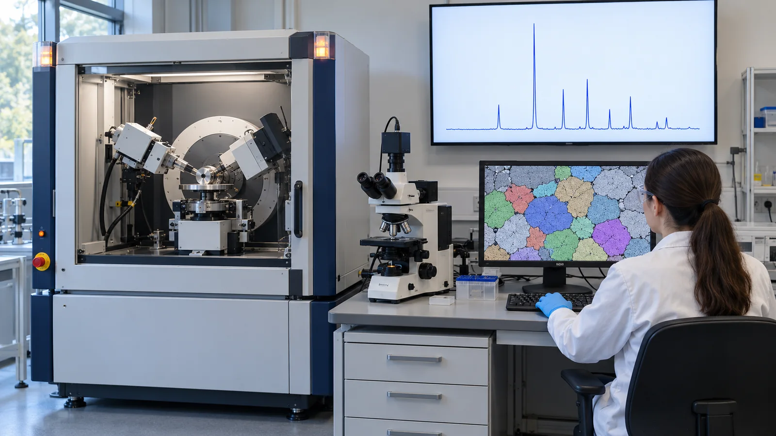
- The short version / before you read / where this sits in the series
- What "reading measured data" means — waveforms, images and AI's three jobs
- Phase identification from XRD — conventional matching versus AI (CNN)
- Where the training data come from — calculated patterns and how they differ from measurements
- Reading accuracy figures together with their conditions
- A case study: the debate over XRD analysis in an autonomous lab
- Spectroscopy (Raman and X-ray absorption)
- Microscopy images — classifying and painting microstructures
- Denoising — without removing what matters
- How data are split, and leakage — our calculation
- A materials engineer's view — preparing your own data, and where people must decide
- Limits, what could not be confirmed, and summary
- How to read the yardsticks and standards
- Glossary
- References
- Claim-to-source audit
Sourced = stated in published material (link given)
Our calculation = a figure this article derived, with the assumptions spelled out
Not yet confirmed = under revision, in preparation or at the proposal stage, so not final
Readings for materials research are marked separately as Commentary. Inference is shown in bold.
The calculation examples in Sections 3, 4, 9 and 10 use synthetic data that we generated (with fixed random seeds). They are not results on real samples or instruments. Accuracy figures from papers are reported together with their conditions; they do not rank methods or research groups, because the conditions differ. The checking date is 22 October 2026. The field moves quickly, so the status of models and standards is as of that date. For the ISO standards we checked numbers, titles and scope only, not the texts.
1. The short version / before you read / where this sits in the series
- AI drafts the "reading" of measured data. It is used to narrow down which crystals are in an XRD pattern (phase identification), to sort a micrograph by microstructure (classification), and to reduce noise Sourced [Ref. 1, 2, 11].
- Accuracy figures can only be read with their conditions. The same "about 90%" means different things depending on whether the data were calculated or measured, how many candidates there were, and whether the split was by sample. In the debate over an autonomous lab's analysis, a manual re-analysis later corrected the counts Sourced [Ref. 5].
- People and experiments do the final checking. AI is a tool that narrows candidates and gives a degree of confidence (a probability). The working assumption is that a person looks again, and adds measurements, when the probability is low or when the phase may not be among the candidates.
All you need is some experience of measuring with XRD or a microscope (or of looking at the results). No machine learning background is required. Keep three ideas in mind first.
- Machine learning = "an approximator that learns trends from past data". It is weak outside the range of its data (extrapolation) and does not understand the laws of physics (see our explainer on machine learning and neural network fundamentals).
- Materials search = "looking for treasure on a vast map". AI is a tool for narrowing where to look. Whether there is treasure (a truly new material) is settled by synthesis and measurement (experiment).
- The division of labor among calculation, experiment and AI: calculation "produces candidates, or reference data, cheaply and quickly"; experiment "checks whether it is really so"; AI "narrows where to look and cuts the effort of reading". This article looks at how the three fit together when analyzing measured data.
In this series on materials informatics (MI), this article deals with using AI on data after it has been measured. Automating the measurement itself is covered in our explainers on autonomous laboratories and on high-throughput experiments and robotic synthesis; how far to trust an AI result is covered in the explainer on uncertainty and applicability domains; reproducibility is covered in the explainer on reading MI results and reproducibility. This article can be read on its own; the necessary background is explained in the text.
2. What "reading measured data" means — waveforms, images and AI's three jobs
Start with an everyday scene. You measure a powder sample by XRD and get a waveform of angle against intensity. What do you do with it? Most likely you compare it in your head with reference data: "this peak position belongs to that phase", "this small bump might be an impurity". With a micrograph, too, you tell regions apart from experience: "this white needle-like part is probably cementite".
This "comparing and telling apart" is the work handed to AI. There are two kinds of data: waveforms (one-dimensional) and images (two-dimensional).
| Data | Typical measurements | What we want to know | Name of AI's job |
|---|---|---|---|
| Waveforms (1-D) | XRD, Raman, infrared, X-ray absorption spectroscopy (XAS) | Which phases, compounds or local structures are present | Identification (guessing what is in it), classification |
| Images (2-D) | Optical microscopy, SEM, TEM | Which microstructure it is, and where the defects and grain boundaries are | Classification, segmentation (painting regions), detection |
| Both | — | We want less noise and background so that what we care about is easier to see | Denoising, correction |
The table is this article's own classification, for orientation.
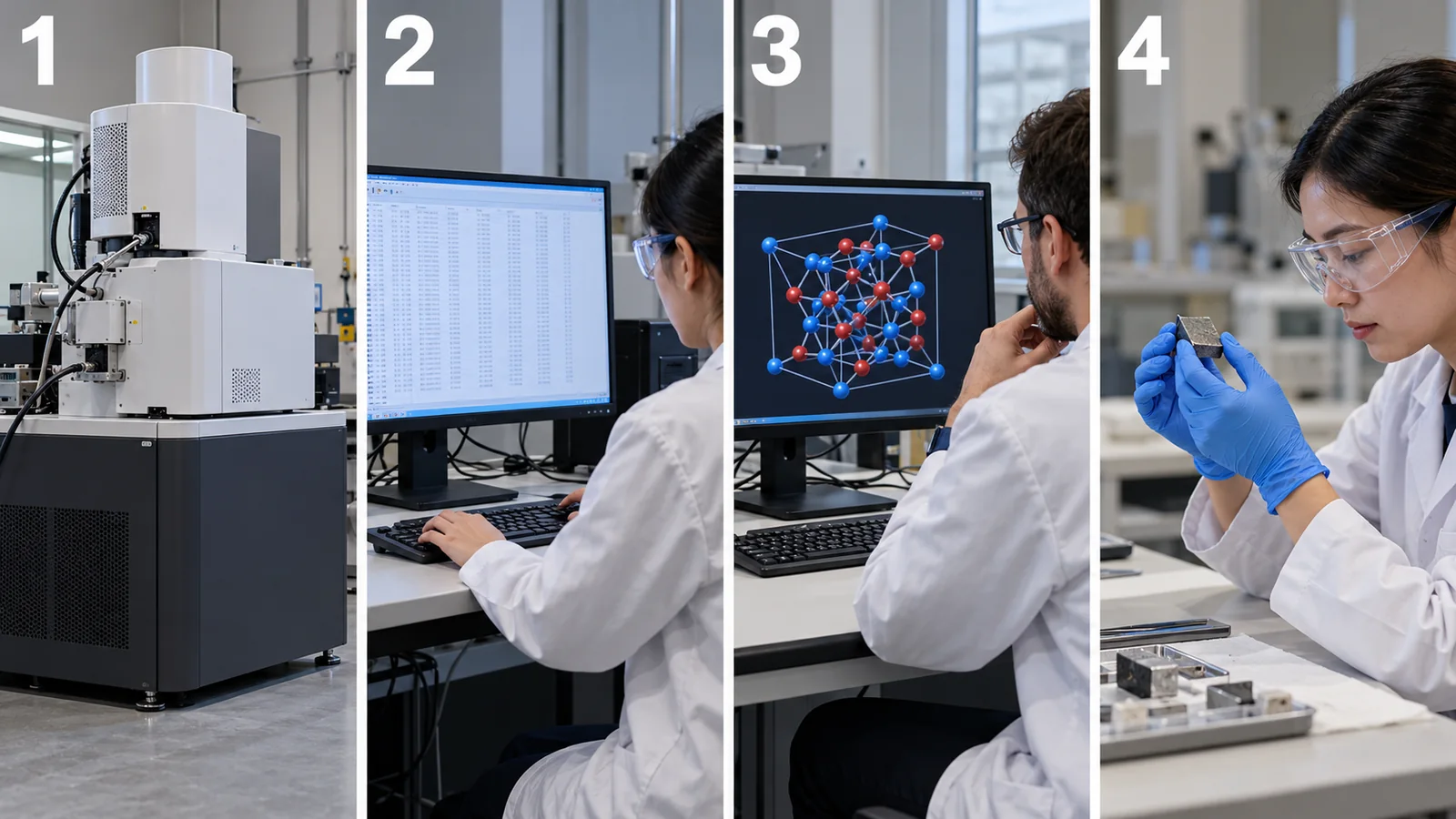
View original SVG, values and sources
Original SVG reference: Concept diagram (vector drawing). How AI reads measured data. AI handles step 3; measurement (step 1) and the final judgment (step 4) remain human and experimental work. The grouping is this article's own arrangement.
Classification gives one answer for the whole sample or image: "which type is this?" Identification answers "what is in it?" (several answers for a mixture). Segmentation paints an image pixel by pixel: "which part is which type?" For example, deciding that "this image is mostly martensite" is classification; painting "this region is martensite and that region is ferrite" is segmentation.
3. Phase identification from XRD — conventional matching versus AI (CNN)
(1) First, why an XRD waveform works like a "fingerprint"
When X-rays hit a crystal, the regular arrangement of atoms produces strong reflections only at particular angles. The angle depends on the spacing d between planes in the crystal and the X-ray wavelength λ (Bragg's law, nλ = 2d sinθ). Because plane spacings differ from substance to substance, the waveform of angle against intensity (the diffraction pattern) acts as the crystal's "fingerprint" (our explanation).
Check it with numbers (Our calculation). The lattice parameter of silicon is about 5.431 Å (the value certified for the NIST reference material is 0.5431109 nm [Ref. 21]). The spacing of the (111) planes is 5.431/√3 ≈ 3.136 Å. With Cu Kα radiation (wavelength 1.5406 Å), sinθ = 1.5406/(2×3.136) gives θ ≈ 14.22°, so the measured angle (2θ) is 28.44°.
A "fingerprint match" is a helpful analogy. A fingerprint helps identify a person. But the analogy has limits: in a mixture, several fingerprints overlap, and where peaks coincide it can become unclear which phase a peak belongs to.
(2) The conventional way: extract peaks and match them
Conventional "phase identification" extracts peak positions and intensities from the measured pattern and compares them with the reference patterns in a standard database (for example the freely available Crystallography Open Database [Ref. 25], or paid databases). Software lists candidates in order of similarity, and a person makes the final choice. Szymanski et al. also use this kind of profile matching as the representative conventional method in their comparison [Ref. 2].
(3) The AI (CNN) way: feed in the whole waveform and output probabilities
The AI approach takes the whole waveform (for example 4,501 intensity values for 2θ from 10° to 80° [Ref. 2]) as input and outputs "how likely each candidate phase is". The model used is a convolutional neural network (CNN).
Think of a CNN as "a device that slides a small window along the waveform, looking for peak-like shapes". The first layer picks up small shapes such as "sharp" or "broad-skirted"; each further layer picks up larger features such as "three peaks at a certain spacing". The difference from the conventional method is that people do not decide which features to pick up; the network learns them from a large number of labelled patterns. Limit of the analogy: the "features" a CNN picks up are not necessarily physical quantities a person can interpret (such as plane spacings). Even when the answer is right, it can be hard to explain why.
In the method of Szymanski et al., the prediction is repeated 1,000 times for the same input (randomly dropping some of the network's connections each time), and the fraction of repeats in which a phase is chosen is treated as its "probability" [Ref. 2]. This probability can serve as a cue for deciding which results a person should review. In that paper, for a test on calculated single-phase patterns, keeping only predictions with a probability above 70% (84% of the whole test set) raised accuracy from 92% to 96% Sourced [Ref. 2]. We could not confirm from the paper whether this probability is calibrated, that is, whether predicted probabilities match how often the answers are actually right.
More detail: why the candidate phases must be fixed in advance
These methods assume that the candidate answers (reference phases) are fixed beforehand. In the evaluation by Szymanski et al., the answer was chosen from 255 reference phases in the Li–Mn–Ti–O–F system (140 stable phases reported in experiments plus 115 hypothetical solid solutions) Sourced [Ref. 2]. If the sample contains a phase that is not among the candidates, the AI answers with "the closest one among the candidates". This is how the general weakness of machine learning at extrapolation shows up in XRD (our explanation).
4. Where the training data come from — calculated patterns and how they differ from measurements
To train AI, you need a large number of pairs of a waveform and its answer (which phase it is). For new materials and thin films, however, labelled measured data hardly exist. So many studies use diffraction patterns calculated from known crystal structures as training data. Oviedo et al. used calculated patterns made from a crystal structure database (ICSD) [Ref. 1], and Szymanski et al. did the same [Ref. 2].
Here is the pitfall. A calculated pattern is for an "ideal crystal", and measurements differ from it in three ways.
- Position shift: strain in a thin film, solid solution (a shift in composition) or a sample sitting at the wrong height moves the peak angles.
- Width change: the smaller the crystal grains (crystallites), the broader the peaks.
- Intensity change: when crystals align in a particular direction (texture), the ratios of peak heights change. This happens especially often in thin films [Ref. 1].
Szymanski et al. added such mismatches to the calculated patterns in advance to enlarge the training set (data augmentation): up to ±4% strain on the lattice parameters, peak widths corresponding to crystallite sizes of 1–100 nm (Scherrer equation), and up to ±50% change in peak intensities. They made 150 patterns per reference phase, 38,250 calculated spectra for 255 phases Sourced [Ref. 2]. Oviedo et al. likewise proposed "physics-informed data augmentation" that accounts for the orientation and lattice strain typical of thin films Sourced [Ref. 1].
The numbers under Fig. 4 (our calculation) give a feel for the size of the mismatches. A 1% change in the lattice parameter alone moves a peak near 28° by about 0.3°. An augmentation of ±4% corresponds to a shift of roughly ±1.1°. Szymanski et al. also report that augmentation cannot cope with changes beyond its range, such as large composition shifts. In their evaluation before adding hypothetical solid solutions to the training, the structure was identified correctly for 11 of 20 calculated patterns (95% after adding them) Sourced [Ref. 2].
The augmentation ranges (±4% strain, 1–100 nm crystallites and so on) are the ranges of samples the authors had in mind. Thin films, powders, sintered bodies and electrode sheets show mismatches differently. An electrode sheet, for example, has peaks from the metal current collector overlapping a broad background from polymers and resins (our commentary). To use such a method on your own samples, the basic step is to re-validate it with training data that reproduce your own typical mismatches (sample holder, texture, background). The most valuable data are those from your own reference samples (known phases) measured on the same instrument under the same conditions. For checking the instrument itself, there are NIST-certified reference materials such as silicon powder SRM 640g [Ref. 21].
5. Reading accuracy figures together with their conditions
"90% accuracy" looks like an easy number. But unless you know what counted as correct, what it was compared against, and what data it was measured on, it has no fixed meaning. Here we read figures from actual papers together with their conditions.
Let us read the figures in Fig. 5 one by one.
| Report | Data (training / evaluation) | Reported figures | Cautions when reading |
|---|---|---|---|
| Oviedo et al. (2019) [1] | Calculated patterns from ICSD plus 115 measured thin-film samples (metal halides; 3 dimensionalities, 7 space groups) | By cross-validation, 93% for dimensionality and 89% for space group. Trained on a small dataset using data augmentation. Accuracy was kept even when the XRD step size was coarsened to 0.16° (2θ), so a pattern could be measured and classified in 5.5 minutes or less Sourced | The test is on a narrow system, thin-film metal halides. 115 samples is few. We could not confirm the details of the cross-validation split from the paper's text |
| Szymanski et al. (2021) [2] (calculated spectra) | 140 phases in the Li–Mn–Ti–O–F system. Calculated patterns with artifacts mixed in; 80% for training, 20% (4,200 patterns) for testing | The CNN reached 94% and the commercial profile-matching software JADE 78% (tests with individual artifacts mixed in). With all artifacts mixed in, CNN 92% and JADE 68% Sourced | The evaluation data are also "made by calculation", like the training data. For measured data see the next row |
| Same (measured spectra) [2] | 10 materials in the same system, measured. Single phases (clean samples, and samples with background, noise, peak shifts, broadening or intensity changes added deliberately) and two- and three-phase mixtures | All 10 clean phases correct. One error among 20 patterns with background (anatase TiO₂). Peak shifts: 5 of 6. Two-phase mixtures 10/10, three-phase 13/15 (JADE 7/10 and 9/15) Sourced | Only 10–20 measurements, so one error moves the figure a lot. The result is for one lab, one instrument and one chemical system |
| Same (calculated mixtures) [2] | 1,000 calculated spectra each: two phases, three phases (equal amounts), and a minor phase (10–30%) | Two-phase 87%, three-phase 78%. For the minor phase alone, 64%; for the major phase, 92% Sourced | Identifying a small impurity phase is hard. Detecting that a second phase is present (the number of phases) is reported at 93%, but that is a different metric from the identification accuracy |
| Earlier work (as described by Szymanski et al.) [2] | Vecsei et al. applied a network trained only on calculated patterns to measured RRUFF mineral spectra | 54% accuracy (as described by Szymanski et al.) Sourced | We did not check the original paper's text. Read it as an example of how training on calculated data alone can drop sharply on measurements |
All figures are as reported in each paper. The table sets side by side figures whose conditions differ; it does not decide which method is better.
The misunderstanding: "The CNN scored 94% and the conventional method (JADE) 78%, so AI is better."
What is correct: This comparison holds under conditions the authors designed (that chemical system, those calculated data, that configuration of JADE). The result could change with JADE's settings or the choice of reference database. The authors also report where the AI is weak. For example, errors are more frequent for low-symmetry monoclinic and triclinic phases, which have many peaks that overlap when broadened (of 113 patterns misclassified because of peak broadening, 82) Sourced [Ref. 2].
Conclusion for use: read the number as "confirmation that the method works under those conditions", and re-measure it on your own samples.
Letting AI decide the next measurement
In a separate paper, Szymanski et al. connected a diffractometer to AI and reported "adaptive XRD", which analyzes results during the measurement and decides which angles to measure carefully next. They showed that small amounts of a material could be detected with short measurement times, and that short-lived intermediate phases during a solid-state reaction could be followed on a standard in-house diffractometer Sourced [Ref. 3]. Combining measurement with AI is covered in our explainers on closed-loop optimization and on autonomous laboratories.
6. A case study: the debate over XRD analysis in an autonomous lab
Claims of accuracy are sometimes revisited later. Here we only set out, neutrally, what has been published. This is not an assessment of any person or research group.
| When | What happened | Label |
|---|---|---|
| November 2023 | Szymanski et al. published a report in Nature on the autonomous laboratory "A-Lab". The paper states that XRD of the powder samples was analyzed by machine-learning models trained on structures from the Materials Project (computed structures) and ICSD, and that the results were confirmed by automated Rietveld refinement. The abstract in the current online version (which reflects the correction described below) reads "36 compounds realized from 57 targets in 17 days" [4] | Sourced |
| 2024 | Leeman et al. (PRX Energy) examined the synthesis products of the A-Lab and pointed to problems in the analysis. They argued that "automated Rietveld analysis of powder XRD data is not yet reliable" and that two thirds of the claimed successful materials are likely to be known compositionally disordered versions of the predicted ordered compounds [6] | Sourced (the critics' claim) |
| 19 January 2026 | The authors published a correction (Nature 650, E1). They revised the wording of the novelty claim, saying the intention, "new to the prediction platform", could be misinterpreted. They re-analyzed the diffraction patterns manually and confirmed 36 of the 40 reported successes, with 4 inconclusive from XRD alone. The re-analysis was peer-reviewed after publication. One compound that had been included in the training data by mistake was removed from the discussion [5] | Sourced (the authors' correction) |
This table is an arrangement of published documents only. We do not judge the merits of the criticism or the correction.
The case shows how heavy the checking must be when an AI analysis result is used for the conclusion "a new phase was made".
- XRD alone may not settle it: a disordered structure in which elements share sites can give a diffraction pattern similar to the ordered structure. Design the work so that another measurement (compositional analysis, electron microscopy, another spectroscopy) backs it up.
- What you put into the references decides the result: if predicted structures are the references, phases similar to the predictions tend to become the answer (our commentary). You need the idea of including disordered solid solutions as candidates too.
- Keep evaluation targets out of the training data: the correction removes a compound that was included in the training data by mistake. This is one real example of the data leakage discussed in Section 10.
7. Spectroscopy (Raman and X-ray absorption)
AI analysis of waveforms is not limited to XRD. Here are two examples, with their conditions.
- Raman spectroscopy (measuring molecular vibrations of a substance): Liu et al. evaluated, on RRUFF (a public database of minerals [Ref. 9]), a method in which a CNN identifies substances from raw Raman spectra without preprocessing such as baseline correction. They report better classification performance than other machine learning, including support vector machines Sourced [Ref. 8]. However, the evaluation is on a mineral database, and we did not confirm specific accuracy figures, or performance on materials other than minerals, beyond what the abstract gives.
- X-ray absorption spectroscopy (XAS, which looks at the local structure around an atom): Torrisi et al. showed that random forests (a method that combines many decision trees) can predict the coordination number around an atom (4-, 5- or 6-fold), the nearest-neighbor distance and the Bader charge (the amount of electron charge assigned to an atom) from several thousand spectra of transition-metal oxides, and examined which spectral regions matter Sourced [Ref. 7]. The spectra used there were not measured but theoretical spectra calculated with FEFF (for computed structures from Materials Project and OQMD) [Ref. 7]. Whether the approach carries over to measured XAS was not tested in that work.
When training data are calculated, they can be made in large numbers, with the answer (local structure) attached. The downside is that whatever differs between calculation and measurement (instrument resolution, sample inhomogeneity, calculation approximations) is not carried over to the AI. How well the bridge to measurements holds must be checked for each method.
8. Microscopy images — classifying and painting microstructures
(1) Classifying microstructures: the steel example of Azimi et al.
Judging a steel's microstructure is work in which an experienced person looks at a micrograph and tells martensite from bainite and so on. Human judgments can contain subjectivity and observer-to-observer differences. Azimi et al. proposed a method that, from SEM images of low-carbon steel, judges the type of each pixel and decides the name of each object by majority vote (Fig. 6). For four microstructure constituents they report an accuracy of 93.94%, above the 48.89% of an earlier method on the same data Sourced [Ref. 11].
What to notice in this figure is how the images were split. In the paper, 11 images were used for training and 10 for testing; in objects, that was 2,831 for training and 2,262 for testing. The split was by image (objects from the same image do not straddle training and test), which prevents the leakage discussed in Section 10. The authors themselves call it a "proof of concept" and leave finer bainite classification (upper, lower and so on) to a next stage Sourced [Ref. 11].
(2) Organizing microstructure images as a "manifold": the ultrahigh-carbon steel of DeCost et al.
DeCost et al. released a dataset of SEM images of ultrahigh-carbon steel microstructures made with various heat treatments. They compared image features (from a method called SIFT, and from a CNN) and tried classifying the main constituent and the annealing condition. They also showed that a dimensionality-reduction method, t-SNE, can visualize the relation between microstructure and processing Sourced [Ref. 12]. A related paper from the same group [Ref. 27] released micrographs of ultrahigh-carbon steel made under various heat treatments together with processing metadata and source code, and showed tools for retrieving similar microstructures from an image and for drawing maps of microstructure and processing conditions Sourced. It is an example of sharing microstructure images together with their conditions.
(3) Atomic-resolution images: counting defects and following motion
Ziatdinov et al. used deep learning to read atom positions, atom types and defect types from scanning transmission electron microscopy (STEM) images in which atoms can be seen. With a "weakly supervised" method that finds even defects absent from the training data from atomic coordinates, they tracked the switching of the coordination of silicon dopant atoms in graphene Sourced [Ref. 10].
(4) Models for painting (segmentation), and pretraining
A representative model for painting images pixel by pixel is U-Net. It was designed to learn from few annotated images by using data augmentation heavily, and it was reported to beat the best prior method in an ISBI challenge on segmenting neuronal structures in electron microscopy stacks Sourced [Ref. 14]. For materials micrographs, "MicroNet" has also been reported: pretrained on more than 100,000 annotated micrographs of 54 material classes. Compared with models pretrained on ImageNet, it generalized better to images taken under different imaging conditions and was more accurate with less training data; when trained on a single image of a nickel superalloy, the relative intersection-over-union (IoU) error fell by 72.2% Sourced [Ref. 13].
IoU (intersection over union) is a measure of how much the region painted by the AI overlaps the region painted correctly by a person: the "overlapping area" divided by the "area of both combined". For example, if the correct region is 100 pixels, the AI's region is 80 pixels and the overlap is 60 pixels, then IoU = 60/(100 + 80 − 60) = 0.5 (Our calculation). Note that the "correct" painting also varies from person to person. Whether an IoU is high has to be read against the variation in the correct answers (our commentary).
9. Denoising — without removing what matters
Measured data carry noise. Reducing noise makes small peaks easier to find and gives AI cleaner input. But telling noise from signal is not simple. Here we check what happens with the simplest method, the moving average, using a small calculation.
(1) Our calculation: stronger smoothing flattens peaks
We add noise to a synthetic waveform (two close peaks of height 100 and 80, and a small peak of height 4) and apply a moving average with different window sizes. Fig. 8 shows the results.
With a small window (5 points), noise falls by about half (1.51 → 0.72) and the peak shapes are largely preserved. When the window equals the peak width (0.30°, 15 points), the taller peak has already lost about 20% of its height (100 → 82). With 41 points (0.82°), the two close peaks nearly become one lump, the valley fills in and the small peak is buried. Our calculation
The method matters even for the same window size. With the method proposed by Savitzky and Golay (fitting a polynomial inside the window and smoothing with it [Ref. 18]), in our calculation a 15-point window with a cubic polynomial kept the shapes well: the two peaks at 99 and 80, the valley at 10.8 and the small peak at 4.1 Our calculation. So a design decision is needed: "if you want to keep peak shapes, choose a method that has a shape-preserving property rather than a plain average" (our commentary).
(2) AI denoising: what is it learning?
Deep-learning denoising also decides "what is signal" from training data. A method that learns from just two noisy observations, without clean answers (Noise2Noise), has been reported Sourced [Ref. 16]. On the other hand, a review of deep learning for image reconstruction names, among the challenges, how to obtain training data, whether unknown structures can be discovered, and the danger of inferring details that are not really there Sourced [Ref. 17]. That review is about fluorescence microscopy, but the thinking also applies to electron micrographs and spectra (our commentary). A review [Ref. 15] gives an overview of deep learning in electron microscopy.
The misunderstanding: a waveform or image that looks cleaner is a more accurate measurement than the original.
What is correct: denoising does not add information; it subtracts components judged to be "probably noise". Subtract too much and signal is lost (Fig. 8); fill in "plausible shapes" the AI has learned and details that do not exist can appear.
How to check: always save the raw data next to the denoised waveform or image, and use for quantification either the raw data or values whose processing effect has been evaluated.
10. How data are split, and leakage — our calculation
The biggest point in reading the figures of Section 5 is whether the data used for evaluation are really different from the data used for training. Consider this scene. You measure the same sample six times. The six patterns are very similar. If five go into training and one into evaluation, the AI only has to identify a "sample it has already seen" and scores higher than its real ability. This is data leakage. In machine-learning-based science in general, leakage has been found in 17 fields, collectively affecting 294 papers Sourced [Ref. 19].
We check with a calculation. Assume three similar crystal types and make ten samples of each. Each sample has its peak positions shifted by ±0.7° (standard deviation) and is measured six times (180 patterns in all). The classification method is a simple one that answers the type of the nearest training pattern (nearest-neighbor). We compare two ways of splitting (Fig. 9).
- A: split measurement by measurement at random (measurements of the same sample can land in both training and test)
- B: split by sample (measurements of one sample go only to training or only to testing)
The result: with A, accuracy was 1.00 in all 30 runs; with B, the mean was 0.75 (0.48 to 1.00). Chance is 0.33. Our calculation. The figure for A is correct only "because the sample was seen during training" and says nothing about the ability on a new sample. Evaluating on "new samples", as in B, is the split closer to real use (measuring unknown samples).
Measurements of the same sample share the sample's quirks (peak shift, crystallite size, texture). These quirks have nothing to do with the crystal type. But if the same sample is in both training and evaluation, the AI can score by the "quirks" rather than the type. In real use, a new sample arrives each time. So evaluation must also be done on "new samples". Likewise, measurements from the same batch, the same day or the same instrument share quirks, so it is safer to split them together (our commentary).
11. A materials engineer's view — preparing your own data, and where people must decide
- Store the measurement conditions with the data: instrument, X-ray source, slits, step size, scan speed, sample holder, sample preparation (grinding, forming, thin film), date and operator. A waveform alone does not tell you the cause of a shift.
- Keep the basis of each label (answer): record who decided "this sample is phase A", and by what (Rietveld refinement, another analysis). If labels contain human disagreement, that disagreement sets the upper limit of AI accuracy.
- Keep failed measurements and strongly shifted ones too: AI trained only on clean data becomes weak against real-world shifts (Section 4). Examples of shifts from your own work are valuable data.
- Evaluate split by lot and by date: as in Section 10, accuracy depends on the split. Holding back "next month's lot" for evaluation is the check closest to real use.
- Check the instrument's yardstick: use a reference material to confirm regularly that peak positions and widths are right for the instrument (for example NIST silicon powder SRM 640g [Ref. 21]). If the instrument drifts, so do the AI's results.
What can be left to AI, and where expert judgment is needed
| Situation | Easier to leave to AI | Needs expert judgment |
|---|---|---|
| Routine phase checks | A first-pass judgment where the phases are known combinations and the probability is high | Low probability, suspicion of a phase not among the candidates, any claim of a new phase |
| Detecting minor phases | A warning that "a second phase may be present" | Identifying the minor phase (accuracy falls [Ref. 2]) and quantifying its content |
| Micrographs | Pre-sorting large numbers of images; rough painting of regions | The final judgment of grain size or microstructure by a standard (for example measurement by the method of ISO 643 [Ref. 23]) |
| Denoising and correction | Display, for visualization | Whether to use it for quantification, and how far processing is acceptable |
The table is this article's own arrangement (commentary).
12. Limits, what could not be confirmed, and summary
(1) Figures whose original text we could not check
The 54% of Vecsei et al. rests on the description in the paper by Szymanski et al.; we did not check the original paper's text. We also did not confirm the specific accuracy of Liu et al. (Raman) beyond the abstract. Ziatdinov et al., Torrisi et al. and DeCost et al. are cited from their titles and abstracts.
(2) Texts of standards
For ISO 16700, ISO 643 and ISO/IEC TS 4213 we checked the number, title, status and scope on the ISO pages. The standards' texts (test conditions, procedures, acceptance criteria) are paid, and we did not check them. For Japanese Industrial Standards on X-ray diffraction analysis (such as JIS K 0131), we could not confirm the number, title or current edition from an official source on the checking date, so they are not stated.
(3) Data and methods not covered
We do not cover neutron diffraction, total scattering (PDF analysis), electron diffraction, EBSD (electron backscatter diffraction), spectral analysis other than deep learning (principal component analysis, non-negative matrix factorization and so on), or spectrum and image analysis with foundation models (very large models).
(4) Companies' products and software
We do not cover the products of instrument makers or analysis-software companies, or claims about their accuracy (we did not check them as primary sources).
(5) Developments in Japan
We did not survey data infrastructure or spectral databases at research institutes in Japan.
- AI drafts the "reading" of measured data. Typical examples are phase identification from XRD, Raman and XAS spectra, classification and painting of micrographs, and denoising Sourced
- Training data are often calculated, and mismatches with measurements are added during training. In thin films, texture and strain matter. A 1% change in the lattice parameter moves a peak near 28° by about 0.3° Sourced / Our calculation
- Read accuracy figures with their conditions. A reported value changes meaning with calculated versus measured data, the range of candidates, the split and the number of measurements. Minor phases and low-symmetry phases are hard Sourced
- When an analysis result is used for a "new" conclusion, make the checking heavier. In the autonomous-lab case, a manual re-analysis corrected the counts Sourced
- The split changes the figure. In our synthetic-data example it was 1.00 for a random split and 0.75 for a split by sample Our calculation
- Denoising subtracts information. Excessive smoothing flattens close peaks Our calculation
13. How to read the yardsticks and standards
How good AI analysis of spectra and images is depends first on four things: the basis of the correct answer (who decided it, and by what), how the evaluation data were split (by sample or by lot), the metric (accuracy, missed minor phases, IoU and so on) and what it is compared against (the baseline). Numbers can be compared only when these are aligned. There are international standards for AI in general, but we could not find a standard that sets "the conditions under which AI may be used for XRD phase identification". Here is what we could confirm (checked 22 October 2026).
| Item evaluated | Representative benchmarks and evaluation methods (name and source) | Standards and guidelines (ISO/IEC, NIST and others) | Cautions when reading |
|---|---|---|---|
| Classification accuracy | Each paper reports on its own evaluation data (for example cross-validation by Oviedo et al. [1], calculated and measured spectra by Szymanski et al. [2], split by image by Azimi et al. [11]) Sourced | ISO/IEC TS 4213:2022 "Information technology — Artificial intelligence — Assessment of machine learning classification performance" (published October 2022; on the ISO page at the "to be revised" stage, with ISO/IEC DIS 4213 listed as the next edition) [24] Sourced Not yet confirmed | We could not confirm a common benchmark. Figures under different conditions cannot be compared |
| Generalization to measured data | RRUFF, a public database of measured Raman, XRD and other data on minerals [9]. An example of training on calculated data only and evaluating on measurements (54%) [2] Sourced | Could not be confirmed | Training on calculated data alone may drop on measurements (Sections 4 and 5) |
| Reference databases | Crystallography Open Database (COD; paper in Nucleic Acids Research, 2012) [25]. The contents of paid databases are not quoted | Could not be confirmed | What you put into the references changes the answer (Section 6) |
| Segmentation and classification of micrographs | IoU and similar. The MicroNet evaluation [13], Warwick electron microscopy datasets [26], UHCSDB (micrographs of ultrahigh-carbon steel) [27] Sourced | Could not be confirmed (we could not find a standard specific to evaluating the accuracy of AI here) | The "correct" painting varies between people. Split by image and by sample |
| Reliability of the XRD instrument | — | NIST SRM 640g (silicon powder; lattice parameter a = 0.5431109 nm, expanded uncertainty ±0.000008 nm (k = 2), at 22.5 °C). NIST SP 260-245 (February 2024) [21] Sourced | A yardstick for calibrating instrument position and width. Not a standard for AI accuracy |
| Magnification calibration of SEM images | — | ISO 16700:2016 "Microbeam analysis — Scanning electron microscopy — Guidelines for calibrating image magnification" (2nd edition, published August 2016; reviewed and confirmed in 2023) [22] Sourced | A precondition when AI measures lengths or grain sizes from images (the magnification must be right) |
| Measuring grain size in steel | — | ISO 643:2024 "Steels — Micrographic determination of the apparent grain size" (5th edition, published August 2024) [23] Sourced | A conventional method that can serve as the comparison when AI measures grain size (our commentary). We could not confirm whether the standard recognizes AI methods |
| Reusability of data | FAIR principles (Wilkinson et al., 2016) [20] Sourced | (FAIR is a set of principles, not an ISO-type standard) | The principles are recommendations, not requirements. They are a reason to store data together with the measurement conditions |
| Checking for data leakage | The taxonomy of leakage and the checklist of Kapoor and Narayanan (2023) [19] Sourced | Could not be confirmed | State the unit of the split and the preprocessing steps in the report |
The arrangement of the table is Our calculation (arrangement). Numbers, titles, editions and status for ISO and NIST were checked on their official pages (22 October 2026). The texts of standards are paid, so only their scope is noted.
Cautions when reading (for materials engineers)
- A ranking in a paper is not the ability on your samples: a paper gives results for the chemical system, instrument and conditions its authors chose. Re-measure with your own reference samples and real samples, split by sample and by lot.
- A prediction (AI's reading) is not experimental confirmation: AI output is "candidates and their likelihoods", not proof that a new phase exists. Design the work so another measurement backs it up (Section 6).
- If AI is trained on calculated data, evaluate on measurements too: a figure evaluated on calculated data depends on how the calculated data were made. Discount a figure that has no evaluation on measurements by that much.
- How strong a principle or standard is: the FAIR principles are recommendations, and ISO/IEC standards are mostly voluntary; they bind only when cited in law or a contract (the latter is our commentary). Plans and standards under revision are treated as Not yet confirmed.
14. Glossary
- XRD (X-ray diffraction)
- A measurement that sends X-rays at a crystal and reads the arrangement of the crystal from the angles and intensities of the reflections.
- Diffraction pattern
- The waveform of angle (2θ) against intensity from XRD. Likened to a crystal's "fingerprint".
- Bragg's law
- The condition for reflection, nλ = 2d sinθ. The angle is set by the plane spacing d and the wavelength λ.
- Phase / phase identification
- A kind of crystal in a sample / finding out what is in it.
- Profile matching
- The conventional method of overlaying a measured pattern on reference patterns and comparing.
- Rietveld refinement
- An analysis that fits a pattern calculated from a crystal-structure model to the measurement.
- CNN (convolutional neural network)
- AI for waveforms and images that slides a small window along the data to pick up local shapes.
- Data augmentation
- Enlarging the training data by adding deformations and shifts to the original data.
- Texture (preferred orientation)
- Crystals aligned in a particular direction. It changes the ratios of peak heights.
- Crystallite / Scherrer equation
- A grain of crystal that scatters X-rays as one unit / an equation estimating crystallite size from peak broadening.
- Raman spectroscopy
- A measurement that shines light on a sample and reads molecular vibrations from the wavelength shift of the scattered light.
- XAS / XANES
- X-ray absorption spectroscopy / its near-edge part, which probes the local structure and electronic state around an atom.
- Random forest
- A machine-learning method that combines many decision trees to predict.
- Classification / segmentation
- Assigning one label to a whole image / painting each pixel by type.
- IoU
- How well an AI region overlaps the correct region (intersection divided by union).
- Pretraining / transfer learning
- Learning first from a large separate dataset, then adjusting to your small dataset.
- Data leakage
- Information that should be used only for evaluation getting into training, which inflates the evaluation.
- Cross-validation
- Splitting data several ways and repeating training and evaluation, then averaging.
- Savitzky–Golay method
- A smoothing method that fits a polynomial inside a window.
- Reference material (SRM)
- A substance with certified values, used to calibrate instruments, such as NIST's silicon powder.
- FAIR principles
- Principles for making data findable, accessible, interoperable and reusable.
- MI (materials informatics)
- Using data, calculation and machine learning to make materials research more efficient.
15. References
- Oviedo F. et al. "Fast and interpretable classification of small X-ray diffraction datasets using data augmentation and deep neural networks", npj Comput. Mater. 5, 60 (2019), DOI 10.1038/s41524-019-0196-x (open access) — nature.com/articles/s41524-019-0196-x
- Szymanski N. J., Bartel C. J., Zeng Y., Tu Q., Ceder G. "Probabilistic Deep Learning Approach to Automate the Interpretation of Multi-phase Diffraction Spectra", Chem. Mater. 33, 4204–4215 (2021), DOI 10.1021/acs.chemmater.1c01071 (the preprint arXiv:2103.16664 was used to check the text) — arxiv.org/abs/2103.16664
- Szymanski N. J. et al. "Adaptively driven X-ray diffraction guided by machine learning for autonomous phase identification", npj Comput. Mater. 9, 31 (2023), DOI 10.1038/s41524-023-00984-y — nature.com/articles/s41524-023-00984-y
- Szymanski N. J. et al. "An autonomous laboratory for the accelerated synthesis of inorganic materials", Nature 624, 86–91 (2023), DOI 10.1038/s41586-023-06734-w — nature.com/articles/s41586-023-06734-w
- Szymanski N. J. et al. "Author Correction: An autonomous laboratory for the accelerated synthesis of inorganic materials", Nature 650, E1 (19 January 2026), DOI 10.1038/s41586-025-09992-y — nature.com/articles/s41586-025-09992-y
- Leeman J. et al. "Challenges in High-Throughput Inorganic Materials Prediction and Autonomous Synthesis", PRX Energy 3, 011002 (2024), DOI 10.1103/PRXEnergy.3.011002 — doi.org/10.1103/PRXEnergy.3.011002
- Torrisi S. B. et al. "Random forest machine learning models for interpretable X-ray absorption near-edge structure spectrum-property relationships", npj Comput. Mater. 6, 109 (2020), DOI 10.1038/s41524-020-00376-6 (open access) — nature.com/articles/s41524-020-00376-6
- Liu J. et al. "Deep convolutional neural networks for Raman spectrum recognition: a unified solution", Analyst 142, 4067–4074 (2017), DOI 10.1039/c7an01371j — doi.org/10.1039/c7an01371j
- RRUFF project "RRUFF Database of Mineral Data" (official site) — rruff.info
- Ziatdinov M. et al. "Deep Learning of Atomically Resolved Scanning Transmission Electron Microscopy Images: Chemical Identification and Tracking Local Transformations", ACS Nano 11, 12742–12752 (2017), DOI 10.1021/acsnano.7b07504 — doi.org/10.1021/acsnano.7b07504
- Azimi S. M. et al. "Advanced Steel Microstructural Classification by Deep Learning Methods", Sci. Rep. 8, 2128 (2018), DOI 10.1038/s41598-018-20037-5 (open access) — nature.com/articles/s41598-018-20037-5
- DeCost B. L., Francis T., Holm E. A. "Exploring the microstructure manifold: Image texture representations applied to ultrahigh carbon steel microstructures", Acta Mater. 133, 30–40 (2017), DOI 10.1016/j.actamat.2017.05.014 (arXiv:1702.01117 was used to check the abstract) — arxiv.org/abs/1702.01117
- Stuckner J. et al. "Microstructure segmentation with deep learning encoders pre-trained on a large microscopy dataset", npj Comput. Mater. 8, 200 (2022), DOI 10.1038/s41524-022-00878-5 (open access) — doi.org/10.1038/s41524-022-00878-5
- Ronneberger O., Fischer P., Brox T. "U-Net: Convolutional Networks for Biomedical Image Segmentation", arXiv:1505.04597 (MICCAI 2015) — arxiv.org/abs/1505.04597
- Ede J. M. "Deep learning in electron microscopy", Mach. Learn.: Sci. Technol. 2, 011004 (2021), DOI 10.1088/2632-2153/abd614 — doi.org/10.1088/2632-2153/abd614
- Lehtinen J. et al. "Noise2Noise: Learning Image Restoration without Clean Data", arXiv:1803.04189 (ICML 2018) — arxiv.org/abs/1803.04189
- Belthangady C., Royer L. A. "Applications, promises, and pitfalls of deep learning for fluorescence image reconstruction", Nat. Methods 16, 1215–1225 (2019), DOI 10.1038/s41592-019-0458-z — doi.org/10.1038/s41592-019-0458-z
- Savitzky A., Golay M. J. E. "Smoothing and Differentiation of Data by Simplified Least Squares Procedures", Anal. Chem. 36, 1627–1639 (1964), DOI 10.1021/ac60214a047 — doi.org/10.1021/ac60214a047
- Kapoor S., Narayanan A. "Leakage and the reproducibility crisis in machine-learning-based science", Patterns 4, 100804 (2023), DOI 10.1016/j.patter.2023.100804 (open access) — doi.org/10.1016/j.patter.2023.100804
- Wilkinson M. D. et al. "The FAIR Guiding Principles for scientific data management and stewardship", Sci. Data 3, 160018 (2016), DOI 10.1038/sdata.2016.18 — doi.org/10.1038/sdata.2016.18
- Cline J. P. et al. "Certification of Standard Reference Material 640g: Line Position and Line Shape Standard for Powder Diffraction (Silicon Powder)", NIST Special Publication 260-245 (February 2024), DOI 10.6028/NIST.SP.260-245 — doi.org/10.6028/NIST.SP.260-245
- ISO "ISO 16700:2016 Microbeam analysis — Scanning electron microscopy — Guidelines for calibrating image magnification" (ISO page) — iso.org/standard/65375.html
- ISO "ISO 643:2024 Steels — Micrographic determination of the apparent grain size" (ISO page) — iso.org/standard/82221.html
- ISO/IEC "ISO/IEC TS 4213:2022 Information technology — Artificial intelligence — Assessment of machine learning classification performance" (ISO page) — iso.org/standard/79799.html
- Gražulis S. et al. "Crystallography Open Database (COD): an open-access collection of crystal structures and platform for world-wide collaboration", Nucleic Acids Res. 40, D420–D427 (2012), DOI 10.1093/nar/gkr900 — doi.org/10.1093/nar/gkr900
- Ede J. M. "Warwick electron microscopy datasets", Mach. Learn.: Sci. Technol. 1, 045003 (2020), DOI 10.1088/2632-2153/ab9c3c — doi.org/10.1088/2632-2153/ab9c3c
- DeCost B. L. et al. "UHCSDB: UltraHigh Carbon Steel Micrograph DataBase", Integr. Mater. Manuf. Innov. 6, 197–205 (2017), DOI 10.1007/s40192-017-0097-0 — link.springer.com/article/10.1007/s40192-017-0097-0
16. Claim-to-source audit
| Claim in the text | Basis | Label |
|---|---|---|
| A CNN that classifies dimensionality and space group from thin-film XRD: calculated patterns plus 115 measured samples, physics-informed data augmentation, 93% for dimensionality and 89% for space group by cross-validation, a step size of 0.16° (5.5 minutes or less) | Abstract and text of Oviedo et al. (2019) Reference 1 https://www.nature.com/articles/s41524-019-0196-x | Sourced |
| The method of Szymanski et al.: physics-informed augmentation of calculated patterns (strain ±4%, crystallites 1–100 nm, intensity ±50%), 255 reference phases (140 + 115), 38,250 patterns, 4,501-point input, probabilities from 1,000 predictions | Szymanski et al. (methods, arXiv version) Reference 2 https://arxiv.org/abs/2103.16664 | Sourced |
| Calculated spectra: CNN 94% and JADE 78% (92% and 68% with artifacts mixed), 92% to 96% above 70% probability, correct phase in the top three for 99%, two-phase 87% and three-phase 78%, minor phase 64% and major phase 92%, 11/20 to 95% after adding solid solutions | Szymanski et al. (results) Reference 2 https://arxiv.org/abs/2103.16664 | Sourced |
| Measured spectra: all 10 clean phases correct, 1 error in 20 patterns with background, peak shifts 5/6, two-phase 10/10 and three-phase 13/15 (JADE 7/10 and 9/15), 82 of 113 errors from peak broadening in monoclinic and triclinic phases | Szymanski et al. (experiments and results) Reference 2 https://arxiv.org/abs/2103.16664 | Sourced |
| 54% reported by Vecsei et al. for a network trained on calculated patterns and applied to measured RRUFF data (as described by Szymanski et al.) | Introduction of Szymanski et al.; original paper not checked Reference 2 https://arxiv.org/abs/2103.16664 | Sourced |
| Adaptive XRD linking measurement and AI: detecting trace phases and following intermediate phases in solid-state reactions | Abstract of Szymanski et al. (2023) Reference 3 https://www.nature.com/articles/s41524-023-00984-y | Sourced |
| A-Lab: XRD analyzed by ML trained on Materials Project and ICSD structures and confirmed by automated Rietveld refinement; the current abstract gives 36 compounds from 57 targets in 17 days | Abstract and text of Szymanski et al. (2023) Reference 4 https://www.nature.com/articles/s41586-023-06734-w | Sourced |
| Author correction (19 January 2026): novelty wording revised; manual re-analysis confirmed 36 of 40 reported successes with 4 inconclusive; re-analysis peer-reviewed after publication; one compound mistakenly in the training data removed | Nature 650, E1 (Author Correction) Reference 5 https://www.nature.com/articles/s41586-025-09992-y | Sourced |
| Critique by Leeman et al.: automated Rietveld analysis not reliable; two thirds of predicted compounds likely known disordered solid solutions (the critics' claim) | Abstract of Leeman et al. (PRX Energy) Reference 6 https://doi.org/10.1103/PRXEnergy.3.011002 | Sourced |
| XANES spectra were calculated with FEFF, and random forests predicted coordination number, nearest-neighbor distance and Bader charge | Abstract and methods of Torrisi et al. (2020) Reference 7 https://www.nature.com/articles/s41524-020-00376-6 | Sourced |
| A CNN identifying substances from Raman spectra without preprocessing, evaluated on RRUFF, with better performance than SVM and others (within the abstract) | Abstract of Liu et al. (2017) Reference 8 https://doi.org/10.1039/c7an01371j Reference 9 https://rruff.info/ | Sourced |
| Deep-learning reading of atom positions, types and defects from STEM images, including defects absent from the training data by a weakly supervised method | Abstract of Ziatdinov et al. (2017) Reference 10 https://doi.org/10.1021/acsnano.7b07504 | Sourced |
| Four low-carbon-steel constituents, 93.94% with per-pixel classification and voting (earlier method 48.89%), split by image (11 for training, 10 for test; 2,831 and 2,262 objects), proof of concept | Abstract and text of Azimi et al. (2018) Reference 11 https://www.nature.com/articles/s41598-018-20037-5 | Sourced |
| A dataset of SEM images of ultrahigh-carbon steel, comparison of SIFT and CNN features, visualization with t-SNE | Abstract of DeCost et al. (2017) Reference 12 https://arxiv.org/abs/1702.01117 Reference 27 https://link.springer.com/article/10.1007/s40192-017-0097-0 | Sourced |
| MicroNet: pretraining on more than 100,000 annotated micrographs (54 classes), generalization to different imaging conditions, 72.2% lower IoU error (trained on one nickel-superalloy image) | Abstract of Stuckner et al. (2022) Reference 13 https://doi.org/10.1038/s41524-022-00878-5 | Sourced |
| U-Net learns from few annotated images and was reported to beat the prior best method on the ISBI segmentation of electron microscopy images | Abstract of Ronneberger et al. Reference 14 https://arxiv.org/abs/1505.04597 | Sourced |
| A review of deep learning in electron microscopy | Abstract of Ede (2021) Reference 15 https://doi.org/10.1088/2632-2153/abd614 | Sourced |
| Noise2Noise: learning from noisy examples only. Challenges of deep-learning image reconstruction (training data, discovering unknown structures, inferring details not there) | Abstracts of Lehtinen et al. and of Belthangady and Royer Reference 16 https://arxiv.org/abs/1803.04189 Reference 17 https://doi.org/10.1038/s41592-019-0458-z | Sourced |
| Smoothing by polynomial fitting (the Savitzky–Golay method) was proposed (title and bibliographic data) | Bibliographic data of Savitzky and Golay (1964) Reference 18 https://doi.org/10.1021/ac60214a047 | Sourced |
| Leakage affected 17 fields and 294 papers in total | Kapoor and Narayanan (2023) Reference 19 https://doi.org/10.1016/j.patter.2023.100804 | Sourced |
| Title and bibliographic data of the FAIR principles (Wilkinson et al., 2016) | Bibliographic data of the paper Reference 20 https://doi.org/10.1038/sdata.2016.18 | Sourced |
| SRM 640g: lattice parameter a = 0.5431109 nm (22.5 °C), expanded uncertainty ±0.000008 nm (k = 2), about 7.5 g of silicon powder, February 2024 | Abstract of NIST SP 260-245 Reference 21 https://doi.org/10.6028/NIST.SP.260-245 | Sourced |
| Number, title and status of ISO 16700:2016 (August 2016, reviewed and confirmed in 2023) and ISO 643:2024 (August 2024) | ISO pages Reference 22 https://www.iso.org/standard/65375.html Reference 23 https://www.iso.org/standard/82221.html | Sourced |
| ISO/IEC TS 4213:2022 (October 2022, at the "to be revised" stage) and the listing of the next edition, ISO/IEC DIS 4213 | ISO page Reference 24 https://www.iso.org/standard/79799.html | Sourced Not yet confirmed |
| Bibliographic data of the COD paper and of the Warwick electron microscopy datasets paper | Bibliographic data of the papers Reference 25 https://doi.org/10.1093/nar/gkr900 Reference 26 https://doi.org/10.1088/2632-2153/ab9c3c | Sourced |
| Silicon (111) at 2θ = 28.44°; changes of −0.29° and −1.12° for lattice parameters +1% and +4%; widths of 0.08°, 0.82° and 8.2° for crystallites of 100, 10 and 1 nm (Scherrer equation, shape factor 0.9); the IoU 0.5 example | Our calculation (Bragg's law and the Scherrer equation; lattice parameter 5.431 Å, wavelength 1.5406 Å). Not a measurement on a real sample | Our calculation |
| The smoothing figures of Fig. 8 (windows of 5, 15 and 41 points; Savitzky–Golay with 15 points and a cubic), and the nearest-neighbor accuracies of Fig. 9 (1.00 and a mean of 0.75, range 0.48 to 1.00) | Our calculation (Python, NumPy; synthetic data, fixed random seeds). Not a measurement on a real sample | Our calculation |
| The current edition of Japanese Industrial Standards such as JIS K 0131, the text of the original paper by Vecsei et al., the specific accuracy of the Raman work, and the calibration of the probabilities | Could not be confirmed in the primary sources accessible within the scope of this survey, so they are not stated | Commentary |
| The readings that "extrapolation is weak", "the way mismatches appear differs by sample", "another measurement must back it up", "choose a method that keeps shape rather than a plain average" and "ISO/IEC standards are mostly voluntary", and the arrangement of what to leave to AI and what experts decide | This article's arrangement and commentary based on published content. Not views stated by any institution | Commentary |
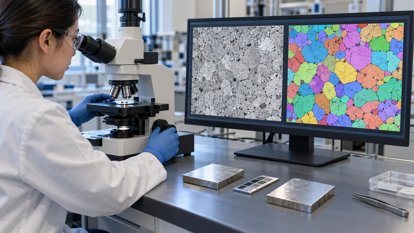
| That Figs. 2 to 6, 8 and 9 are explanatory drawings, not real observations, and that Figs. 1 and 7 are ImageGen-generated conceptual illustrations | Note by this article | Commentary |
Last updated 22 October 2026. Sources are limited to primary material (peer-reviewed papers, arXiv papers, and NIST and ISO official pages). The texts of ISO standards are paid and could not be checked. The calculation examples are on synthetic data that we generated, not results on real samples. The current edition of Japanese Industrial Standards such as JIS K 0131, the text of the original paper by Vecsei et al., the specific accuracy of the Raman work, and the calibration of the probabilities could not be confirmed and are not stated here. All figures are explanatory concept graphics or drawings that include our calculations. Figs. 1 and 7 are ImageGen-generated conceptual illustrations, and none of them shows a real instrument or measurement result.